Daten und Zeiten sind keine einfachen Objekte:

Monate enthalten eine andere Anzahl von Tagen;
Jahre sind Schaltjahre und nicht;
Es gibt verschiedene Zeitzonen.
Stunden, Minuten, Tage verwenden unterschiedliche Zahlensysteme;
und viele andere Nuancen.

Im Folgenden finden Sie eine Zusammenfassung einiger Punkte, die in der Dokumentation nur selten hervorgehoben werden, sowie Tricks, mit denen Sie schnellen und kontrollierten Code schreiben können.

Eine sehr kurze Zusammenfassung für Smartphone-Leser: Bei großen Datenmengen verwenden wir nur POSIXct

Sekundenbruchteile. Es wird natürlich schnell gut.

Es ist eine Fortsetzung einer Reihe früherer Veröffentlichungen .

Standards für die Angabe von Daten und Zeiten

ISO 8601 Datenelemente und Austauschformate - Informationsaustausch - Die Darstellung von Datum und Uhrzeit ist eine internationale Norm für den Austausch von datums- und zeitbezogenen Daten.

Grundlegende R-Methoden zum Arbeiten mit der Zeit

Datum

Sys.Date()
print("-----")

x <- as.Date("2019-01-29") #  UTC
print(x)
tz(x)
str(x)
dput(x)

print("-----")
dput(as.Date("1970-01-01")) # ! origin

Konsolenausgabe

## [1] "2021-04-29"
## [1] "-----"
## [1] "2019-01-29"
## [1] "UTC"
##  Date[1:1], format: "2019-01-29"
## structure(17925, class = "Date")
## [1] "-----"
## structure(0, class = "Date")

Nicht standardmäßiges Datumsformat während der Initialisierung muss speziell angegeben werden

as.Date("04/20/2011", format = "%m/%d/%Y")

## [1] "2011-04-20"

Zeit

Es gibt zwei grundlegende Arten von Zeit, die in R verwendet werden: POSIXct

und POSIXlt

.

Die Außenansichten POSIXct

und POSIXlt

sehen ähnlich aus. Und die internen?

z <- Sys.time()
glue(" ", 
     "POSIXct - {z}", 
     "POSIXlt - {as.POSIXlt(z)}", "---", .sep = "\n")

glue(" ", 
     "POSIXct - {capture.output(dput(z))}", 
     "POSIXlt - {paste0(capture.output(dput(as.POSIXlt(z))), collapse = '')}",
     "---", .sep = "\n")

#    /  
glue(": {year(z)} \n: {minute(z)}\n: {second(z)}\n---")

Konsolenausgabe

##  
## POSIXct - 2021-04-29 15:18:04
## POSIXlt - 2021-04-29 15:18:04
## ---
##  
## POSIXct - structure(1619698684.50764, class = c("POSIXct", "POSIXt"))
## POSIXlt - structure(list(sec = 4.50764489173889, min = 18L, hour = 15L,     mday = 29L, mon = 3L, year = 121L, wday = 4L, yday = 118L,     isdst = 0L, zone = "MSK", gmtoff = 10800L), class = c("POSIXlt", "POSIXt"), tzone = c("", "MSK", "MSD"))
## ---
## : 2021 
## : 18
## : 4
## ---

Wir kommen sofort zu dem Schluss, dass wir bei ernsthafter Arbeit mit Daten (mehr als 10 Zeilen mit der Zeit) POSIXlt

dies als schlechten Traum vergessen. Es ist eine komplexe Struktur mit wahnsinnigem Overhead.

POSIXct

unixtimestamp, () ( 0 01.01.1970). .

— online unixtimestamp:

z <- 1548802400
as.POSIXct(z, origin = "1970-01-01")                # local
as.POSIXct(z, origin = "1970-01-01", tz = "UTC")    # in UTC

## [1] "2019-01-30 01:53:20 MSK"
## [1] "2019-01-29 22:53:20 UTC"

. . :

ISO, (ISO 8601-2019);
- ;
.

POSIXct

, - . :

x <- ymd_hms("2014-09-24 15:23:10")
x
x + 0.5
x + 0.5 + 0.6

options(digits.secs=5)
x + 0.45756
options(digits.secs=0)
x

## [1] "2014-09-24 15:23:10 UTC"
## [1] "2014-09-24 15:23:10 UTC"
## [1] "2014-09-24 15:23:11 UTC"
## [1] "2014-09-24 15:23:10.45756 UTC"
## [1] "2014-09-24 15:23:10 UTC"

, .

options(digits.secs=5)

# generate data
df <- data.frame(
  timestamp = as_datetime(
    round(runif(20, min = now() - seconds(10), max = now()), 0), 
    tz ="Europe/Moscow")) %>%
  mutate(ms = round(runif(n(), 0, 999), 0)) %>%
  mutate(value = round(runif(n(), 0, 100), 0))

dput(df)

#  " "
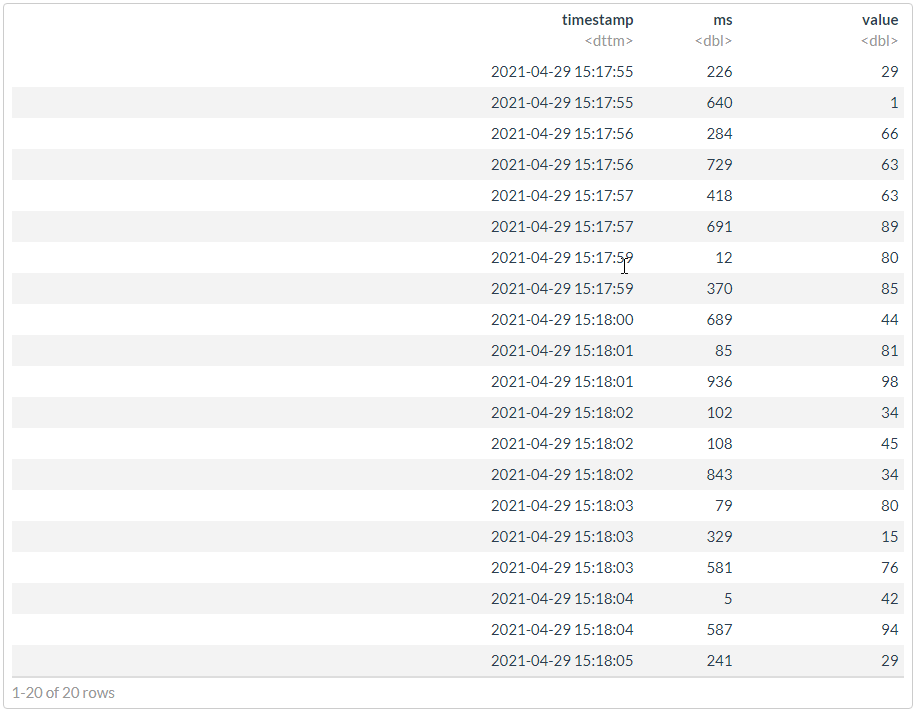
df %>%
  arrange(timestamp, ms)
options(digits.secs=0)

## structure(list(timestamp = structure(c(1619698677, 1619698680, 
## 1619698676, 1619698682, 1619698675, 1619698682, 1619698679, 1619698679, 
## 1619698684, 1619698683, 1619698684, 1619698677, 1619698682, 1619698683, 
## 1619698675, 1619698676, 1619698685, 1619698681, 1619698683, 1619698681
## ), class = c("POSIXct", "POSIXt"), tzone = "Europe/Moscow"), 
##     ms = c(418, 689, 729, 108, 226, 843, 12, 370, 5, 581, 587, 
##     691, 102, 79, 640, 284, 241, 85, 329, 936), value = c(63, 
##     44, 63, 45, 29, 34, 80, 85, 42, 76, 94, 89, 34, 80, 1, 66, 
##     29, 81, 15, 98)), class = "data.frame", row.names = c(NA, 
## -20L))

# "" 
# [magrittr aliases](https://magrittr.tidyverse.org/reference/aliases.html)
df2 <- df %>%
  mutate(timestamp = timestamp + ms/1000) %>%
  # mutate_at("timestamp", ~`+`(. + ms/1000)) %>%
  select(-ms) %>%

df2 %>% arrange(timestamp)

#  
dt <- as.data.table(df2)
bench::mark(
  naive = dplyr::arrange(df, timestamp, ms),
  smart = dplyr::arrange(df2, timestamp),
  dt = dt[order(timestamp)],
  check = FALSE,
  relative = TRUE,
  min_iterations = 1000
)

## # A tibble: 3 x 6
##   expression   min median `itr/sec` mem_alloc `gc/sec`
##   <bch:expr> <dbl>  <dbl>     <dbl>     <dbl>    <dbl>
## 1 naive       11.9   11.8      1         1.06     1   
## 2 smart       11.1   11.0      1.06      1        1.06
## 3 dt           1      1       11.6     494.       1.22

data <- c("05102019210003657", "05102019210003757", "05102019210003857")

dmy_hms(stri_c(stri_sub(data, to = 14L), ".", stri_sub(data, from = 15L)), tz = "Europe/Moscow")

#    
data2 <- data %>%
  sample(10^6, replace = TRUE)
bench::mark(
  stri_sub = stri_c(stri_sub(data2, to = 14L), ".", stri_sub(data2, from = 15L)),
  stri_replace = stri_replace_first_regex(data2, pattern = "(^.{14})(.*)", replacement = "$1.$2"),
  re2_replace = re2_replace(data2, pattern = "(^.{14})(.*)", replacement = "\\1.\\2", parallel = TRUE)
)

## [1] "2019-10-05 21:00:03 MSK" "2019-10-05 21:00:03 MSK"
## [3] "2019-10-05 21:00:03 MSK"
## # A tibble: 3 x 6
##   expression        min   median `itr/sec` mem_alloc `gc/sec`
##   <bch:expr>   <bch:tm> <bch:tm>     <dbl> <bch:byt>    <dbl>
## 1 stri_sub        214ms    222ms      4.10   22.89MB     5.47
## 2 stri_replace    653ms    653ms      1.53    7.63MB     0   
## 3 re2_replace     409ms    413ms      2.42   15.29MB     1.21

`lubridate`

x <- ymd(20101215)
print(x)
class(x)

## [1] "2010-12-15"
## [1] "Date"

lubridate

ymd(20101215) == mdy("12/15/10")

## [1] TRUE

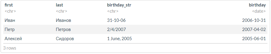
df <- tibble(first = c("", "", ""),
             last = c("", "", ""),
             birthday_str = c("31-10-06", "2/4/2007", "1 June, 2005")) %>%
  mutate(birthday = dmy(birthday_str))

df

, ?

#      lubridate
options(lubridate.verbose = TRUE)
#   : ..
df <- tibble(time_str = c("08.05.19 12:04:56", "09.05.19 12:05", "12.05.19 23"))

lubridate::dmy_hms(df$time_str, tz = "Europe/Moscow")
print("---------------------")
lubridate::dmy(df$time_str, tz = "Europe/Moscow")

## [1] "2019-05-08 12:04:56 MSK" NA                       
## [3] NA                       
## [1] "---------------------"
## [1] NA NA NA

#      lubridate
options(lubridate.verbose = TRUE)

lubridate::dmy_hms(df$time_str, truncated = 3, tz = "Europe/Moscow")

## [1] "2019-05-08 12:04:56 MSK" "2019-05-09 12:05:00 MSK"
## [3] "2019-05-12 23:00:00 MSK"

#      lubridate
options(lubridate.verbose = TRUE)
#   : ..
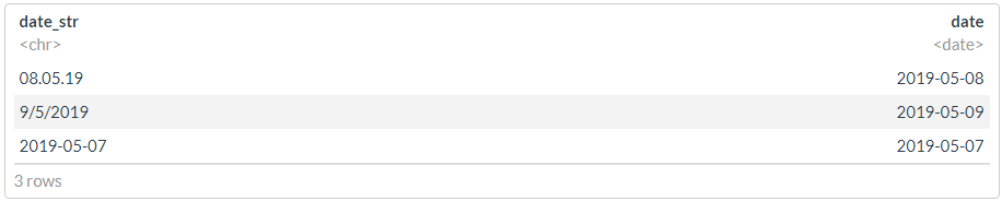
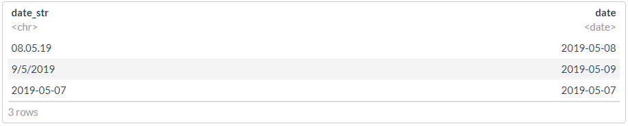
df <- tibble(date_str = c("08.05.19", "9/5/2019", "2019-05-07"))

#   
glimpse(dmy(df$date_str))
print("---------------------")
#   
glimpse(ymd(df$date_str))
print("---------------------")

##  Date[1:3], format: "2019-05-08" "2019-05-09" NA
## [1] "---------------------"
##  Date[1:3], format: "2008-05-19" NA "2019-05-07"
## [1] "---------------------"

? , , , - .

df %>%
  mutate(date = dplyr::coalesce(dmy(date_str), ymd(date_str)))

tab4

df1 <- df
df1$date <- dmy(df1$date_str)
idx <- is.na(df1$date)
print("---------------------")
idx
df1$date[idx] <- ymd(df1$date_str[idx])

print("---------------------")
df1

## [1] "---------------------"
## [1] FALSE FALSE  TRUE
## [1] "---------------------"

tab5

"" :

POSIXct

options(lubridate.verbose = FALSE)
date1 <- ymd_hms("2011-09-23-03-45-23")
date2 <- ymd_hms("2011-10-03-21-02-19")

#     ?
as.numeric(date2) - as.numeric(date1) #   ,   
(date2 - date1) %>% dput()

difftime(date2, date1)
difftime(date2, date1, unit="mins")
difftime(date2, date1, unit="secs")

## [1] 926216
## structure(10.7200925925926, class = "difftime", units = "days")
## Time difference of 10.72009 days
## Time difference of 15436.93 mins
## Time difference of 926216 secs

date1 <- ymd_hms("2019-01-30 00:00:00")

date1

date1 - days(1)
date1 + days(1)
date1 + days(2)

## [1] "2019-01-30 UTC"
## [1] "2019-01-29 UTC"
## [1] "2019-01-31 UTC"
## [1] "2019-02-01 UTC"

—

date1 - months(1)
date1 + months(1) # !!!

## [1] "2018-12-30 UTC"
## [1] NA

. , .

date1 %m-% months(1)
date1 %m+% months(1)
date1 %m+% months(1) %m-% months(1)

## [1] "2018-12-30 UTC"
## [1] "2019-02-28 UTC"
## [1] "2019-01-28 UTC"

date1 <- ymd_hms("2019-01-30 01:00:00")

date1 %T>% print() %>% dput()

with_tz(date1, tzone = "Europe/Moscow") %T>% print() %>% dput()
force_tz(date1, tzone = "Europe/Moscow") %T>% print() %>% dput()

## [1] "2019-01-30 01:00:00 UTC"
## structure(1548810000, class = c("POSIXct", "POSIXt"), tzone = "UTC")
## [1] "2019-01-30 04:00:00 MSK"
## structure(1548810000, class = c("POSIXct", "POSIXt"), tzone = "Europe/Moscow")
## [1] "2019-01-30 01:00:00 MSK"
## structure(1548799200, class = c("POSIXct", "POSIXt"), tzone = "Europe/Moscow")

, , ? , hms

. .

hms_str <- "03:22:14"
as_hms(hms_str)
dput(as_hms(hms_str))
print("-------")

x <- as_hms(hms_str) * 15
x
str(x)
# seconds_to_period(period_to_seconds(x))
seconds_to_period(x) %T>% dput() %>% print()

## 03:22:14
## structure(12134, units = "secs", class = c("hms", "difftime"))
## [1] "-------"
## Time difference of 182010 secs
##  'difftime' num 182010
##  - attr(*, "units")= chr "secs"
## new("Period", .Data = 30, year = 0, month = 0, day = 2, hour = 2, 
##     minute = 33)
## [1] "2d 2H 33M 30S"

— . .

( Clickhouse) , , unixtimestamp UTC. , .

. timestamp, , , , , .
( ). , , , .
unixtimestamp UTC , . (!).
, timestamp. ,

X-1

X+1

, .

, 0.

.

(, ) . , :

, ;
;
;
( );
;
double

;
;
.

--  ClickHouse
SELECT DISTINCT
    store, pos,
    timestamp, ms,
    concat(toString(store), '-', toString(pos)) AS pos_uid,
    toFloat64(timestamp) + (ms / 1000)          AS timestamp

flog.info(paste("SQL query:", sql_req))
tic("  CH")
raw_df <- dbGetQuery(conn, stri_encode(sql_req, to = "UTF-8")) %>%
  mutate_if(is.character, `Encoding<-`, "UTF-8") %>%
  as_tibble() %>%
  mutate_at(vars(timestamp), anytime::anytime, tz = "Europe/Moscow") %>%
  mutate_at("event", as.factor)
flog.info(capture.output(toc()))

DBI::dbDisconnect(conn)

data.frame

#    
df -> as_tibble(_df) %>%
  map(pryr::object_size) %>% 
  unlist() %>% 
  enframe() %>% 
  arrange(desc(value)) %>%
  mutate_at("value", fs::as_fs_bytes) %>%
  mutate(ratio = formattable::percent(value / sum(value), 2)) %>%
  add_row(name = "TOTAL", value = sum(.$value))

, , , . .

df <- seq.Date(from = as.Date("2021-01-01"), 
               to = as.Date("2021-05-31"), 
               by = "2 days") %>%
  # sample(20, replace = FALSE) %>%
  tibble(date = .)

#    // 
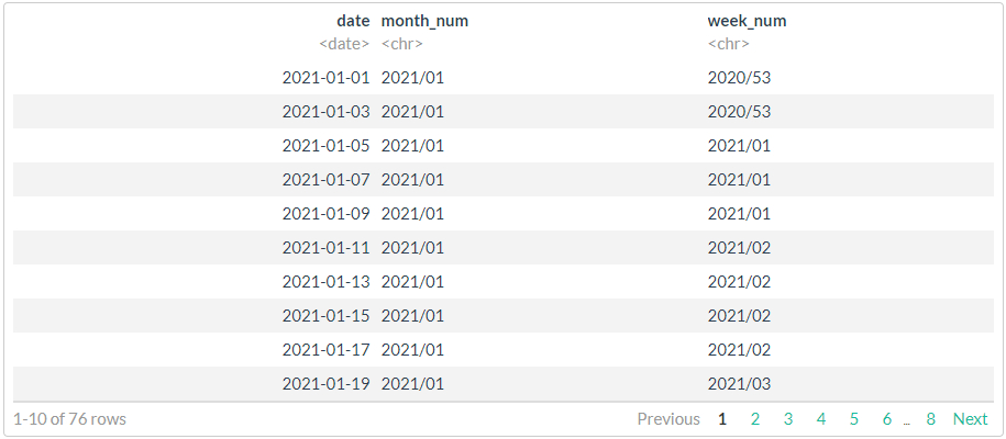
#  1
df %>%
  mutate(month_num = stri_c(lubridate::year(date), 
                            sprintf("%02d", lubridate::month(date)), 
                            sep = "/"),
         week_num = stri_c(lubridate::isoyear(date), 
                           sprintf("%02d", lubridate::isoweek(date)), 
                           sep = "/")
  )

tab6

#    // 
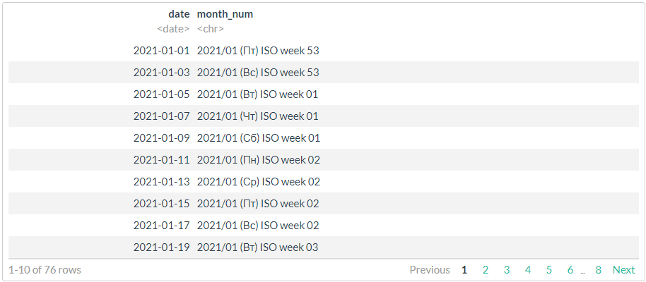
#  2,    

#   ,       !!!
df %>%
  mutate(month_num = format(date, "%Y/%m (%a) ISO week %V"))

tab7

#    // 
#  3,    
#     strptime (ISO 8601)  ICU
# https://man7.org/linux/man-pages/man3/strptime.3.html
stri_datetime_fstr("%Y/%m (%a) week %V")
# ggthemes::tableau_color_pal("Tableau 20")(20) %>% scales::show_col()

#   ,      !!!
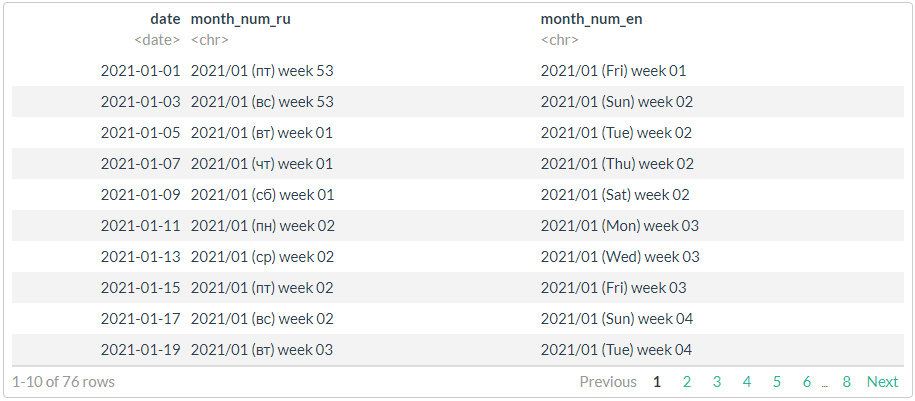
df %>%
  mutate(
    month_num_ru = stri_datetime_format(
      date, "yyyy'/'MM' ('ccc') week 'ww", locale = "ru", tz = "UTC"),
    month_num_en = stri_datetime_format(
      date, "yyyy'/'MM' ('ccc') week 'ww", locale = "en", tz = "UTC"))

tab8

. .

stri_datetime_format(today(), "LLLL", locale="ru@calendar=Persian")
stri_datetime_format(today(), "LLLL", locale="ru@calendar=Indian")
stri_datetime_format(today(), "LLLL", locale="ru@calendar=Hebrew")
stri_datetime_format(today(), "LLLL", locale="ru@calendar=Islamic")
stri_datetime_format(today(), "LLLL", locale="ru@calendar=Coptic")
stri_datetime_format(today(), "LLLL", locale="ru@calendar=Ethiopic")
stri_datetime_format(today(), "dd MMMM yyyy", locale="ru")
stri_datetime_format(today(), "LLLL d, yyyy", locale="ru")

## [1] ""
## [1] ""
## [1] ""
## [1] ""
## [1] ""
## [1] ""
## [1] "29  2021"
## [1] " 29, 2021"

#   
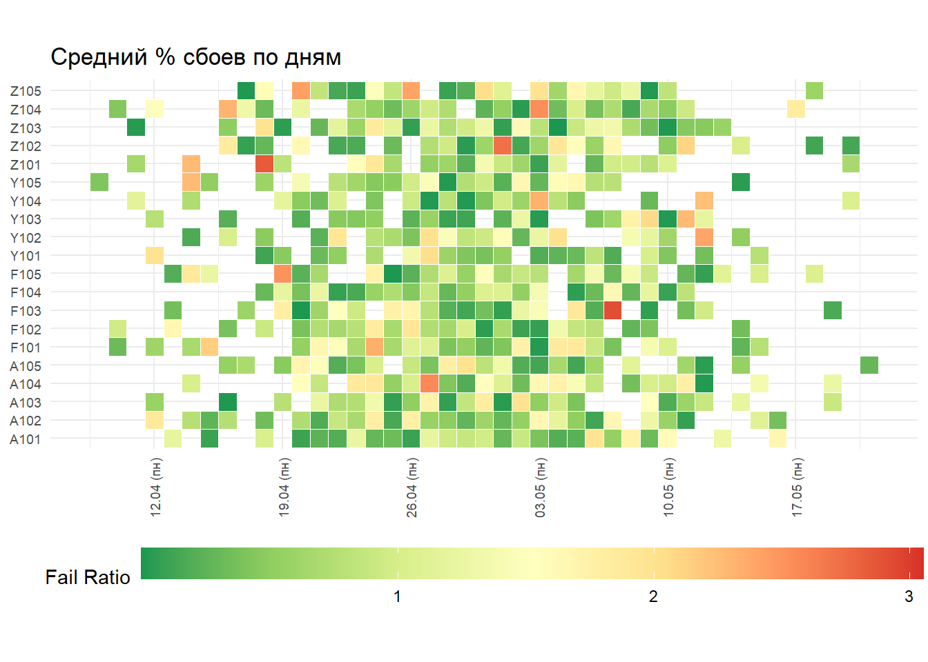
map_tbl <- tibble(
  date = as_date(Sys.time() + rnorm(10^3, mean = 0, sd = 60 * 60 * 24 * 7))) %>%
  mutate(store = stri_c(sample(c("A", "F", "Y", "Z"), n(), replace = TRUE),
                        sample(101:105, n(), replace = TRUE))) %>%
  mutate(store_fct = as.factor(store)) %>%
  mutate(fail_ratio = abs(rnorm(n(), mean = 0.3, sd = 1)))

my_date_format <- function (format = "dd MMMM yyyy", tz = "Europe/Moscow") 
{
  scales:::force_all(format, tz)
  # stri_datetime_fstr("%d.%m%n%A")
  # stri_datetime_fstr("%d.%m (%a)")
  function(x) stri_datetime_format(x, format, locale = "ru", tz = tz)
}

#   ,     
gp <- map_tbl %>%
  ggplot(aes(x = date, y = store_fct, fill = fail_ratio)) +
  geom_tile(color = "white", size = 0.1) +
  # scale_fill_distiller(palette = "RdYlGn", name = "Fail Ratio", label = comma) +
  # scale_fill_distiller(palette = "RdYlGn", name = "Fail Ratio", guide = guide_legend(keywidth = unit(4, "cm"))) +
  scale_fill_distiller(palette = "RdYlGn", name = "Fail Ratio") +
  scale_x_date(breaks = scales::date_breaks("1 week"), labels = my_date_format("dd'.'MM' ('ccc')'")) +
  coord_equal() +
  labs(x = NULL, y = NULL, title = " %   ") +
  theme_minimal() +
  theme(plot.title = element_text(hjust = 0)) +
  theme(axis.ticks = element_blank()) +
  theme(axis.text = element_text(size = 7)) +
  theme(axis.text.x = element_text(angle = 90, vjust = 0.5)) +
  theme(legend.position = "bottom") +
  theme(legend.key.width = unit(3, "cm"))

gp

Heatmap

base_df <- tibble(
  start = Sys.time() + rnorm(10^3, mean = 0, sd = 60 * 24 * 3)) %>%
  mutate(finish = start + rnorm(n(), mean = 100, sd = 60)) %>%
  mutate(user_id = sample(as.character(1000:1100), n(), replace = TRUE)) %>%
  arrange(user_id, start)

dt <- as.data.table(base_df, key = c("user_id", "start")) %>%
  .[, c("start", "finish") := lapply(.SD, as.numeric), 
    .SDcols = c("start", "finish")]

df <- group_by(base_df, user_id)

bench::mark(
  dplyr_v1 = df %>% transmute(delta_t = as.numeric(difftime(finish, start, units = "secs"))) %>% ungroup(),
  dplyr_v2 = ungroup(df) %>% transmute(delta_t = as.numeric(difftime(finish, start, units = "secs"))),
  dplyr_v3 = dt %>% transmute(delta_t = finish - start),
  dt_v1 = dt[, .(delta_t = finish - start), by = user_id],
  dt_v2 = dt[, .(delta_t = finish - start)],
  check = FALSE # all_equal   
)

## # A tibble: 5 x 6
##   expression      min   median `itr/sec` mem_alloc `gc/sec`
##   <bch:expr> <bch:tm> <bch:tm>     <dbl> <bch:byt>    <dbl>
## 1 dplyr_v1      4.3ms   4.86ms      200.   103.1KB    11.4 
## 2 dplyr_v2     2.17ms   2.46ms      380.    17.9KB     6.24
## 3 dplyr_v3     1.67ms   1.77ms      527.    29.8KB     8.51
## 4 dt_v1       410.4us  438.7us     2139.    90.8KB     8.35
## 5 dt_v2       304.4us  335.3us     2785.   264.6KB     8.38

: //. , , ?

Beispielcode. Vergessen Sie nicht, dass eine Reihe von Funktionen unter Berücksichtigung des Gebietsschemas der Maschine funktionieren, auf der der Code ausgeführt wird. Und wenn Ihr Monat in russischer Sprache gedruckt ist, garantiert dies kein ähnliches Verhalten auf einem anderen Computer oder einem anderen Betriebssystem (wenn Sie keine Methoden verwenden).

# https://stackoverflow.com/questions/16347731/how-to-change-the-locale-of-r
# https://jangorecki.gitlab.io/data.cube/library/stringi/html/stringi-locale.html

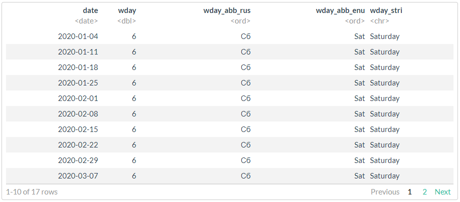
df <- as.Date("2020-01-01") %>% 
  seq.Date(to = . + months(4), by = "1 day") %>%
  tibble(date = .) %>%
  mutate(wday = lubridate::wday(date, week_start = 1),
         wday_abb_rus = lubridate::wday(date, label = TRUE, week_start = 1),
         wday_abb_enu = lubridate::wday(date, label = TRUE, week_start = 1, locale = "English"),
         wday_stri = stringi::stri_datetime_format(date, "EEEE", locale = "en"))

#   
filter(df, wday == 6)

tab9

PS Die meisten Tests sind nur zum Beispiel. Sie können es auf Ihren Maschinen ausführen, die Zahlen sind völlig unterschiedlich, aber die Art der Abhängigkeit und des Verhältnisses sollte ungefähr gleich sein.

Vorheriger Beitrag - "R vs Python in einer produktiven Schleife" .

R und arbeiten im Laufe der Zeit. Was ist hinter den Kulissen?

Standards für die Angabe von Daten und Zeiten

Grundlegende R-Methoden zum Arbeiten mit der Zeit

Datum

Zeit

`lubridate`

POSIXct

More articles:

R und arbeiten im Laufe der Zeit. Was ist hinter den Kulissen?

Standards für die Angabe von Daten und Zeiten

Grundlegende R-Methoden zum Arbeiten mit der Zeit

Datum

Zeit

lubridate (adsbygoogle = window.adsbygoogle || []).push({}); (adsbygoogle = window.adsbygoogle || []).push({}); (adsbygoogle = window.adsbygoogle || []).push({});

POSIXct

More articles:

`lubridate`