👧🏼 🤳🏾 👩🏾‍🌾 Obszöne Anwendung 😗 🈷️ 📆

Ausgeschnittene Materialien finden Sie im Anhang des Artikels zum Partikelpfad : Pfadintegrale, ein Doppelspaltexperiment an kalten Neonatomen, Rahmen der Partikelteleportation und andere Szenen von Grausamkeit und sexueller Natur.

Meiner Meinung nach gibt es keinen anderen Weg, den mathematischen Formalismus als logisch konsistent anzusehen, als zu zeigen, dass seine Konsequenzen von der Erfahrung abweichen, oder zu beweisen, dass seine Vorhersagen die Beobachtungsmöglichkeiten nicht ausschöpfen.

Niels Bohr

Abschließend möchte der Autor feststellen, dass wir nur zwei gute Gründe für die Ablehnung einer Theorie erkennen, die eine Vielzahl von Phänomenen erklärt. Erstens ist die Theorie intern nicht konsistent und zweitens stimmt sie nicht mit Experimenten überein.

David Bohm

Zuvor haben wir gelernt, woher die Schrödinger-Gleichung kommt, warum sie von dort genommen wird und wie sie mit verschiedenen Methoden genommen wird.

i ℏ \frac{\partial Ψ}{\partial t} = (- \frac{ℏ^{2}}{2 m} \nabla^{2} + V) Ψ

$i\hbar\frac{\partial\Psi}{\partial t} = \left( -\frac{\hbar^2}{2m}\nabla^2 + V\right) \Psi$

Teilen wir es nun in zwei reelle Gleichungen auf. Stellen Sie sich dazu psi in polarer Form vor $\Psi = Re^{iS/\hbar}$ , :

\frac{\partial S}{\partial t} + \frac{(\nabla S)^{2}}{2 m} - \frac{ℏ^{2}}{2 m} \frac{\nabla^{2} R}{R} + V = 0 \frac{\partial R^{2}}{\partial t} + \nabla \cdot (\frac{R^{2} \nabla S}{m}) = 0

$\frac{\partial S}{\partial t}+\frac{(\nabla S)^{2}}{2 m}-\frac{\hbar^{2}}{2 m} \frac{\nabla^{2} R}{R}+V=0 \\ \frac{\partial R^{2}}{\partial t}+\nabla \cdot\left(\frac{R^{2} \nabla S}{m}\right)=0$

S — , R — . , , , — -, ( ).

, $U = \nabla S /m$ . , S -, - - :

S = - \frac{i ℏ}{2} \ln \frac{Ψ}{Ψ^{*}}

$S = -\frac{i\hbar}{2}\ln\frac{\Psi}{\Psi^*}$

, -, , , , S, , , , . , , . -.

— , . , , , . , , , .

, , , . . . , , , .

, .

, , , . , ( - ). :

()

, , , : ,

, . . .

U = \nabla S / m = - \frac{i ℏ}{2 m} \nabla \ln \frac{Ψ}{Ψ^{*}} = \frac{ℏ}{m} I m (\frac{\nabla ψ}{ψ})

$U = \nabla S /m = -\frac{i\hbar}{2m}\nabla\ln\frac{\Psi}{\Psi^*} = \frac{\hbar}{m}\mathrm{Im}\left(\frac{\nabla\psi}{\psi} \right)$

-, :

x + = U Δ t

$x += U\Delta t$

using LinearAlgebra, SparseArrays, Plots

const ħ = 1.0546e-34 # J*s
const m = 9.1094e-31 # kg
const q = 1.6022e-19 # Kl
const nm = 1e-9 # m
const fs = 1e-12; # s

function wavefun()

    gauss(x) = exp( -(x-x0)^2 / (2*σ^2) + im*x*k )
    k = m*v/ħ

    #    
    Vm = spdiagm(0 => V )
    H = spdiagm(-1 => ones(Nx-1), 0 => -2ones(Nx), 1 => ones(Nx-1) )
    H *= ħ^2 / ( 2m*dx^2 )
    H += Vm

    A = I + 0.5im*dt/ħ * H #  
    B = I - 0.5im*dt/ħ * H # 
    psi = zeros(Complex, Nx, Nt)
    psi[:,1] = gauss.(x)

    for t = 1:Nt-1

        b = B * psi[:,t]
        #       A*psi = b
        psi[:,t+1] = A \ b
    end

    return psi
end

dx = 0.05nm # x step
dt = 0.01fs # t step
xlast = 400nm
Nt = 260 # Number of time steps
t = range(0, length = Nt, step = dt)

x = [0:dx:xlast;]
Nx = length(x) # Number of spatial steps

a1 = 200nm
a2 = 200.5nm # 5 
a3 = 205nm
a4 = 205.5nm 
#V = [ a1<xi<a2 ? 2q : 0.0 for xi in x ] # 2 eV 
V = [ a1<xi<a2 || a3<xi<a4 ? 2q : 0.0 for xi in x ] # 2 eV 

x0 = 80nm # Initial position
σ = 20nm # gauss width
v = -120nm/fs;

@time Psi = wavefun()
P = abs2.(Psi);

function ψ(xi, j)

    k = findfirst(el-> abs(el-xi)<dx, x)
    k == nothing && ( k = 1 )

    Psi[k, j]
end

function corpusculaz(n)

    X = zeros(n, Nt)
    X[:,1] = x0 .+ σ*randn(n)

    for j in 2:Nt, i in 1:n
        U = ħ/(2m*dx) * imag( ( ψ(X[i,j-1]+dx, j) -  ψ(X[i,j-1]-dx, j) ) /  ψ(X[i,j-1], j) )
        X[i,j] = X[i,j-1] - U*dt
    end

    X
end

@time X = corpusculaz(20);

plot(x, P[:, 1], legend = false)
plot!(x, P[:, 80], legend = false)
scatter!( X[:,1], zeros(20) )
scatter!( X[:,80], zeros(20) )

. — , . :

, . , , !

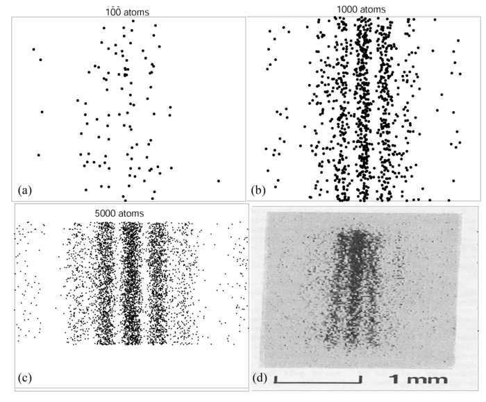
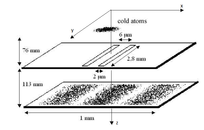
, . Double-slit interference with ultracold metastable neon atoms — - .

using Random, Gnuplot, Statistics
#  
function trapez(f, a, b, n)
    h = (b - a)/n
    result = 0.5*(f(a) + f(b))
    for i in 1:n-1
        result += f(a + i*h)
    end
    result * h
end
#  
function rk4(f, x, y, h)
    k1 = h * f(x       , y        )
    k2 = h * f(x + 0.5h, y + 0.5k1)
    k3 = h * f(x + 0.5h, y + 0.5k2)
    k4 = h * f(x +    h, y +    k3)

    return y + (k1 + 2*(k2 + k3) + k4)/6.0
end

const ħ = 1.055e-34 # J*s 
const kB = 1.381e-23 # J*K-1
const g = 9.8 # m/s^2

const l1 = 76e-3 # m
const l2 = 113e-3 # m
const yh = 2.8e-3 # m
const d = 6e-6 # m
const b = 2e-6 # m
const a1 = 0.5(- d - b) # 
const a2 = 0.5(- d + b)
const b1 = 0.5(  d - b)
const b2 = 0.5(  d + b)

const m = 3.349e-26 # kg
const T = 2.5e-3 # K
const σv = sqrt(kB*T/m) #  
const σ₀ = 10e-6 # 10 mkm #      
const σz = 3e-4 # 0.3 mm #  z
const σk = m*σv / (ħ*√3) # 2e8 m/s #    

v₀ = zeros(3)
k₀ = zeros(3);

: , , -, .

\begin{aligned} 1) ψ_{0} (x, y, z; k_{0 x}, k_{0 y}, k_{0 z}) = & ψ_{0 x} (x; k_{0 x}) ψ_{0_{y}} (z; k_{0 y}) ψ_{0 z} (z; k_{0 z}) \\ = & {(2 π σ_{0}^{2})}^{- 1 / 4} e^{- x^{2} / 4 σ_{0}^{2}} e^{i k_{0 x} x} \\ \times {(2 π σ_{0}^{2})}^{- 1 / 4} e^{- y^{2} / 4 σ_{0}^{2}} e^{i k_{0 y} y} \\ \times {(2 π σ_{z}^{2})}^{- 1 / 4} e^{- z^{2} / 4 σ_{z}^{2}} e^{i k_{0 z} z} \end{aligned}

$\begin{aligned} 1)\psi_{0}\left(x, y, z ; k_{0 x}, k_{0 y}, k_{0 z}\right)=& \psi_{0 x}\left(x ; k_{0 x}\right) \psi_{0_{y}}\left(z ; k_{0 y}\right) \psi_{0 z}\left(z ; k_{0 z}\right) \\ =&\left(2 \pi \sigma_{0}^{2}\right)^{-1 / 4} e^{-x^{2} / 4 \sigma_{0}^{2}} e^{i k_{0 x} x} \\ & \times\left(2 \pi \sigma_{0}^{2}\right)^{-1 / 4} e^{-y^{2} / 4 \sigma_{0}^{2}} e^{i k_{0 y} y} \\ & \times\left(2 \pi \sigma_{z}^{2}\right)^{-1 / 4} e^{-z^{2} / 4 \sigma_{z}^{2}} e^{i k_{0 z} z} \end{aligned}$

, . , , , . , , .

, . , , — . , , , . , , .

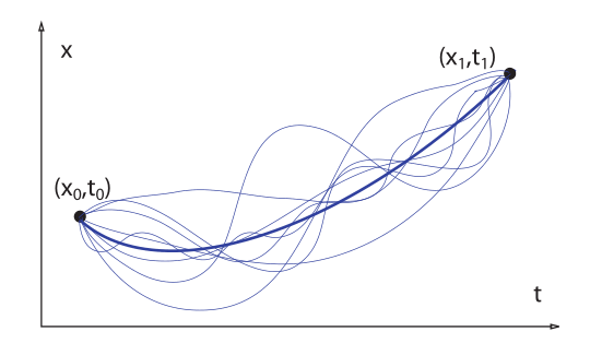
Quantum Mechanics And Path Integrals, A. R. Hibbs, R. P. Feynman, , 3.6 .

K (β, t_{β}; α, t_{α}) = K_{x} (x_{β}, t_{β}; x_{α}, t_{α}) K_{y} (y_{β}, t_{β}; y_{α}, t_{α}) K_{z} (z_{β}, t_{β}; z_{α}, t_{α})

$K\left(\beta, t_{\beta} ; \alpha, t_{\alpha}\right)=K_{x}\left(x_{\beta}, t_{\beta} ; x_{\alpha}, t_{\alpha}\right) K_{y}\left(y_{\beta}, t_{\beta} ; y_{\alpha}, t_{\alpha}\right) K_{z}\left(z_{\beta}, t_{\beta} ; z_{\alpha}, t_{\alpha}\right)$

\begin{aligned} K_{x} (x_{β}, t_{β}; x_{α}, t_{α}) = & {(\frac{m}{2 i π ℏ (t_{β} - t_{α})})}^{1 / 2} \exp \frac{i m}{ℏ} (\frac{{(x_{β} - x_{α})}^{2}}{2 (t_{β} - t_{α})}) \\ K_{y} (y_{β}, t_{β}; y_{α}, t_{α}) = & {(\frac{m}{2 i π ℏ (t_{β} - t_{α})})}^{1 / 2} \exp \frac{i m}{ℏ} (\frac{{(y_{β} - y_{α})}^{2}}{2 (t_{β} - t_{α})}) \\ K_{z} (z_{β}, t_{β}; z_{α}, t_{α}) = & {(\frac{m}{2 i π ℏ (t_{β} - t_{α})})}^{1 / 2} \exp \frac{i m}{ℏ} (\frac{{(z_{β} - z_{α})}^{2}}{2 (t_{β} - t_{α})}) \\ \times \exp \frac{i m}{ℏ} (\frac{g}{2} (z_{β} + z_{α}) (t_{β} - t_{α}) - \frac{g^{2}}{24} {(t_{β} - t_{α})}^{3}) \end{aligned}

$\begin{aligned} K_{x}\left(x_{\beta}, t_{\beta} ; x_{\alpha}, t_{\alpha}\right)=&\left(\frac{m}{2 i \pi \hbar\left(t_{\beta}-t_{\alpha}\right)}\right)^{1 / 2} \exp \frac{i m}{\hbar}\left(\frac{\left(x_{\beta}-x_{\alpha}\right)^{2}}{2\left(t_{\beta}-t_{\alpha}\right)}\right) \\ K_{y}\left(y_{\beta}, t_{\beta} ; y_{\alpha}, t_{\alpha}\right)=&\left(\frac{m}{2 i \pi \hbar\left(t_{\beta}-t_{\alpha}\right)}\right)^{1 / 2} \exp \frac{i m}{\hbar}\left(\frac{\left(y_{\beta}-y_{\alpha}\right)^{2}}{2\left(t_{\beta}-t_{\alpha}\right)}\right) \\ K_{z}\left(z_{\beta}, t_{\beta} ; z_{\alpha}, t_{\alpha}\right)=&\left(\frac{m}{2 i \pi \hbar\left(t_{\beta}-t_{\alpha}\right)}\right)^{1 / 2} \exp \frac{i m}{\hbar}\left(\frac{\left(z_{\beta}-z_{\alpha}\right)^{2}}{2\left(t_{\beta}-t_{\alpha}\right)}\right) \\ & \times \exp \frac{i m}{\hbar}\left(\frac{g}{2}\left(z_{\beta}+z_{\alpha}\right)\left(t_{\beta}-t_{\alpha}\right)-\frac{g^{2}}{24}\left(t_{\beta}-t_{\alpha}\right)^{3}\right) \end{aligned}$

Z , . ,

ψ (β, t) = \int K (β, t; α, t_{α}) ψ (α, t_{α}) d x_{α}, d y_{α}, d z_{α}

$\psi\left(\beta, t \right)=\int K\left(\beta, t ; \alpha, t_{\alpha}\right) \psi\left(\alpha, t_{\alpha}\right) d x_{\alpha}, d y_{\alpha}, d z_{\alpha}$

, . , X, . :

\begin{aligned} ψ_{x} (x, t; k_{0 x}) & = \int K (x, t; x_{α}, 0) ψ_{0} (x_{α}) d x_{α} \\ ψ_{x} (x, t; k_{0 x}) & = {(2 π s_{0}^{2} (t))}^{- 1 / 4} \exp [- \frac{{(x - v_{0 x} t)}^{2}}{4 σ_{0} s_{0} (t)} + i k_{0 x} (x - v_{0 x} t)] \\ ρ_{x} (x, t) & = {(2 π ε_{0}^{2} (t))}^{- 1 / 2} \exp [- \frac{x^{2}}{2 ε_{0}^{2} (t)}] \end{aligned}

$\begin{aligned} \psi_{x}\left(x, t ; k_{0 x}\right)&=\int K\left(x, t ; x_\alpha, 0\right) \psi_0\left(x_\alpha\right) d x_{\alpha}\\ \psi_{x}\left(x, t ; k_{0 x}\right) &=\left(2 \pi s_{0}^{2}(t)\right)^{-1 / 4} \exp \left[-\frac{\left(x-v_{0 x} t\right)^{2}}{4 \sigma_{0} s_{0}(t)}+i k_{0 x}\left(x-v_{0 x} t\right)\right] \\ \rho_{x}(x, t) &=\left(2 \pi \varepsilon_{0}^{2}(t)\right)^{-1 / 2} \exp \left[-\frac{x^{2}}{2 \varepsilon_{0}^{2}(t)}\right] \end{aligned}$

ε_{0}^{2} (t) = σ_{0}^{2} (t) + {(\frac{h t σ_{v}}{m})}^{2} σ_{0}^{2} (t) = σ_{0}^{2} + {(\frac{h t}{2 m σ_{0}^{2}})}^{2}

$\varepsilon_{0}^{2}(t)=\sigma_{0}^{2}(t)+\left(\frac{h t \sigma_v}{m}\right)^{2}\\ \sigma_{0}^{2}(t)=\sigma_{0}^{2}+\left(\frac{h t}{2 m \sigma_{0}^{2}}\right)^{2}$

, :

ε₀(t) = σ₀^2 + ( ħ/(2m*σ₀) * t )^2 + (ħ*t*σv/m)^2
s₀(t) = σ₀ + im*ħ/(2m*σ₀) * t

ρₓ(x, t) = exp( -x^2 / (2ε₀(t)) ) / sqrt( 2π*ε₀(t) )

t₁(v, z) = sqrt( 2*(l1-z)/g + (v/g)^2 ) - v/g
tf1 = t₁(v₀[3], 0) # s #    
X1 = range(-100, stop = 100, length = 100)*1e-6 
Z1 = range(0, stop = l1, length = 100)
Cron1 = range(0, stop = tf1, length = 100)

P1 = [ ρₓ(x, t) for t in Cron1, x in X1 ]
P1 /= maximum(P1); #   

@gp "set title 'Wavefun before the slits'" xlab="Z, mkm" ylab="X, mkm"
@gp :- 1000Z1 1000000X1 P1 "w image notit"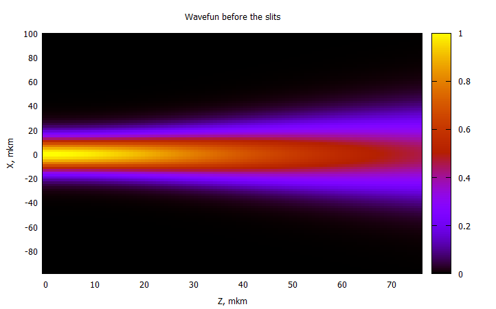

— .

, :

\begin{aligned} ψ_{x} & (x, t) = ψ_{A} + ψ_{B} \\ ψ_{A} & = \int_{A} K_{x} (x, t; x_{a}, t_{1}) ψ_{x} (x_{a}, t_{1}, k_{0 x}) d x_{a} \\ ψ_{B} & = \int_{B} K_{x} (x, t; x_{b}, t_{1}) ψ_{x} (x_{b}, t_{1}, k_{0 x}) d x_{b} \end{aligned}

$\begin{aligned} \psi_{x}&\left(x, t\right)=\psi_{A}+\psi_{B}\\ \psi_{A} &=\int_{A} K_{x}\left(x, t ; x_{a}, t_{1}\right) \psi_{x}\left(x_{a}, t_{1}, k_{0 x}\right) d x_{a} \\ \psi_{B} &=\int_{B} K_{x}\left(x, t ; x_{b}, t_{1}\right) \psi_{x}\left(x_{b}, t_{1}, k_{0 x}\right) d x_{b} \end{aligned}$

ρ_{x} (x, t) = \int_{- \infty}^{+ \infty} {(2 π σ_{v}^{2})}^{- 1 / 2} \exp (- \frac{k_{0 x}^{2}}{2 σ_{v}^{2}}) {| ψ_{x} (x, t; k_{0 x}) |}^{2} d k_{0 x}

$\rho_{x}\left(x, t\right)=\int_{-\infty}^{+\infty}\left(2 \pi \sigma_v^{2}\right)^{-1 / 2} \exp \left(-\frac{k_{0 x}^{2}}{2 \sigma_v^{2}}\right)\left|\psi_{x}\left(x, t ; k_{0 x}\right)\right|^{2} d k_{0 x}$

, :

function ρₓ(xᵢ, tᵢ) 

    Kₓ(xb, tb, xa, ta) = sqrt( m/(2im*π*ħ*(tb-ta)) ) * exp( im*m*(xb-xa)^2 / (2ħ*(tb-ta)) )

    function subintrho(k) 

        ψₓ(x, t) = ( 2π*s₀(t) )^-0.25 * exp( -(x-ħ*k*t/m)^2 / (4σ₀*s₀(t)) + im*k*(x-ħ*k*t/m) )
        subintpsi(x) = Kₓ(xᵢ, tᵢ, x, tf1) * ψₓ(x, tf1)

        ψa = trapez(subintpsi, a1, a2, 200)
        ψb = trapez(subintpsi, b1, b2, 200)

        exp( -k^2 / (2σv^2) ) * abs2(ψa + ψb)
    end

    trapez(subintrho, -10σk, 10σk, 20) / sqrt( 2π*σv^2 )
end

t₂(v, z) = sqrt( 2*(l1+l2-z)/g + (v/g)^2 ) - v/g
tf2 = t₂(v₀[3], 0) # s #    
X2 = range(-800, stop = 800, length = 200)*1e-6
Z2 = range(l1, stop = l2, length = 100)
Cron2 = range(tf1, stop = tf2, length = 100)

@time P2 = [ ρₓ(x, t) for t in Cron2, x in X2 ];

P2 /= maximum(P2[4:end,:]);
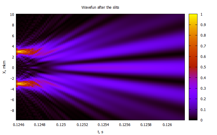
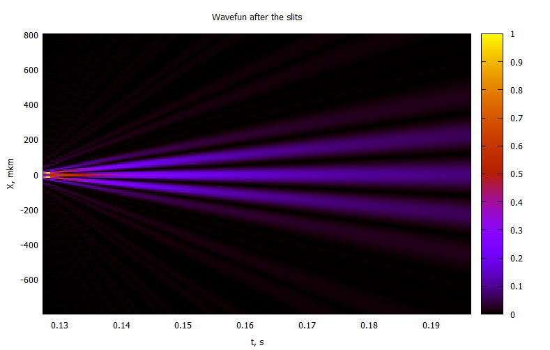
@gp "set title 'Wavefun after the slits'" xlab="t, s" ylab="X, mkm"
@gp :- Cron2[4:end] 1000000X2 P2[4:end,:] "w image notit"

2 :

\vec{v} = \frac{\nabla S}{m}

$\vec v = \frac{\nabla S}{m}$

. . , ,

\begin{aligned} \vec{v} (x, y, z, t) & = \frac{\nabla S}{m} + \frac{\nabla \log ρ \times \vec{s}}{m} \\ \vec{s} & = (0, 0, ℏ / 2) \\ \frac{\nabla \log ρ \times \vec{s}}{m} & = \frac{ℏ}{2 m ρ} (\frac{\partial ρ}{\partial y}, - \frac{\partial ρ}{\partial x}, 0) \end{aligned}

$\begin{aligned} \vec v(x, y, z, t)&=\frac{\nabla S}{m}+\frac{\nabla \log \rho \times \vec s}{m} \\ \vec s &= (0,0,\hbar/2)\\ \frac{\nabla \log \rho \times \vec s}{m} &= \frac{\hbar}{2 m \rho}\left( \frac{\partial \rho}{\partial y}, -\frac{\partial \rho}{\partial x}, 0\right) \end{aligned}$

, ,

\begin{aligned} \frac{d x}{d t} & = v_{x} (x, t) = \frac{1}{m} \frac{\partial S}{\partial x} + \frac{ℏ}{2 m ρ} \frac{\partial ρ}{\partial y} = v_{0 x} + \frac{(x - v_{0 x} t) ℏ^{2} t}{4 m^{2} σ_{0}^{2} σ_{0}^{2} (t)} - \frac{ℏ (y - v_{0 y} t)}{2 m σ_{0}^{2} (t)} \\ \frac{d y}{d t} & = v_{y} (x, t) = \frac{1}{m} \frac{\partial S}{\partial y} - \frac{ℏ}{2 m ρ} \frac{\partial ρ}{\partial x} = v_{0 y} - \frac{(y - v_{0 y} t) ℏ^{2} t}{4 m^{2} σ_{0}^{2} σ_{0}^{2} (t)} + \frac{ℏ (x - v_{0 x} t)}{2 m σ_{0}^{2} (t)} \\ \frac{d z}{d t} & = v_{z} (z, t) = \frac{1}{m} \frac{\partial S}{\partial z} = v_{0 z} + g t + \frac{(z - v_{0 z} t - g t^{2} / 2) ℏ^{2} t}{4 m^{2} σ_{z}^{2} σ_{z}^{2} (t)} \end{aligned}

$\begin{aligned} \frac{d x}{d t} &=v_{x}(x, t)=\frac{1}{m} \frac{\partial S}{\partial x}+\frac{\hbar}{2 m \rho} \frac{\partial \rho}{\partial y}=v_{0 x}+\frac{\left(x-v_{0 x} t\right) \hbar^{2} t}{4 m^{2} \sigma_{0}^{2} \sigma_{0}^{2}(t)}-\frac{\hbar\left(y-v_{0 y} t\right)}{2 m \sigma_{0}^{2}(t)} \\ \frac{d y}{d t} &=v_{y}(x, t)=\frac{1}{m} \frac{\partial S}{\partial y}-\frac{\hbar}{2 m \rho} \frac{\partial \rho}{\partial x}=v_{0 y}-\frac{\left(y-v_{0 y} t\right) \hbar^{2} t}{4 m^{2} \sigma_{0}^{2} \sigma_{0}^{2}(t)}+\frac{\hbar\left(x-v_{0 x} t\right)}{2 m \sigma_{0}^{2}(t)} \\ \frac{d z}{d t} &= v_{z}(z, t)=\frac{1}{m} \frac{\partial S}{\partial z}=v_{0 z}+g t+\frac{\left(z-v_{0 z} t-g t^{2} / 2\right) \hbar^{2} t}{4 m^{2} \sigma_{z}^{2} \sigma_{z}^{2}(t)} \end{aligned}$

\begin{aligned} x (t) & = v_{0 x} t + \sqrt{x_{0}^{2} + y_{0}^{2}} \frac{σ_{0} (t)}{σ_{0}} \cos φ (t) \\ y (t) & = v_{0 y} t + \sqrt{x_{0}^{2} + y_{0}^{2}} \frac{σ_{0} (t)}{σ_{0}} \sin φ (t) \\ z (t) & = v_{0 z} t + \frac{1}{2} g t^{2} + z_{0} \frac{σ_{z} (t)}{σ_{z}} \end{aligned}

$\begin{aligned} x(t) &=v_{0 x} t+\sqrt{x_{0}^{2}+y_{0}^{2}} \frac{\sigma_{0}(t)}{\sigma_{0}} \cos \varphi(t) \\ y(t) &=v_{0 y} t+\sqrt{x_{0}^{2}+y_{0}^{2}} \frac{\sigma_{0}(t)}{\sigma_{0}} \sin \varphi(t)\\ z(t) &= v_{0 z} t+\frac{1}{2} g t^{2}+z_{0} \frac{\sigma_{z}(t)}{\sigma_{z}} \end{aligned}$

\begin{aligned} σ_{0}^{2} (t) & = σ_{0}^{2} + {(\frac{ℏ t}{2 m σ_{0}})}^{2} \\ φ (t) & = φ_{0} + \arctan (- \frac{ℏ t}{2 m σ_{0}^{2}}) \\ \cos (φ_{0}) & = \frac{x_{0}}{\sqrt{x_{0}^{2} + y_{0}^{2}}} \\ \sin (φ_{0}) & = \frac{y_{0}}{\sqrt{x_{0}^{2} + y_{0}^{2}}} \\ \sin (\arctan x) & = \frac{x}{\sqrt{1 + x^{2}}} \\ \cos (\arctan x) & = \frac{1}{\sqrt{1 + x^{2}}} \\ \cos (a + b) & = \cos a \cos b - \sin a \sin b \\ \sin (a + b) & = \sin a \cos b + \cos a \sin b \end{aligned}

$\begin{aligned} \sigma_{0}^{2}(t) &= \sigma_{0}^{2}+\left(\frac{\hbar t}{2 m \sigma_{0}}\right)^{2} \\ \varphi(t) &= \varphi_{0}+\arctan \left(-\frac{\hbar t}{2 m \sigma_{0}^{2}}\right) \\ \cos \left(\varphi_{0}\right) &= \frac{x_{0}}{\sqrt{x_{0}^{2}+y_{0}^{2}}} \\ \sin \left(\varphi_{0}\right) &= \frac{y_{0}}{\sqrt{x_{0}^{2}+y_{0}^{2}} } \\ \sin(\arctan x) &= \frac{x}{\sqrt{1+x^2}} \\ \cos(\arctan x) &= \frac{1}{\sqrt{1+x^2}} \\ \cos(a+b) &= \cos a\cos b - \sin a\sin b \\ \sin(a+b) &= \sin a\cos b + \cos a\sin b \end{aligned}$

function xbs(t, xo, yo, vo)

    cosϕ = xo / sqrt( xo^2 + yo^2 )
    sinϕ = yo / sqrt( xo^2 + yo^2 )
    atnx = -ħ*t / (2m*σ₀^2)
    sinatnx = atnx / sqrt( atnx^2 + 1)
    cosatnx =    1 / sqrt( atnx^2 + 1)
    cosϕt = cosϕ * cosatnx - sinϕ * sinatnx
    #sinϕt = sinϕ*cosatnx + cosϕ*sinatnx

    σ₀t = sqrt( σ₀^2 + ( ħ*t / (2*m*σ₀) )^2 )

    vo*t + sqrt(xo^2 + yo^2) * σ₀t/σ₀ * cosϕt
end

@gp "set title 'Trajectories before slits'" xlab="t, s" ylab="X, mkm" # "set yrange [-10:10]"

@time for i in 1:80

    x0 = randn()*σ₀
    y0 = randn()*σ₀
    v0 = randn()*σv*1e-4

    prtclᵢ = [ xbs(t,x0,y0,v0) for t in Cron1 ]

    @gp :- Cron1 1000000prtclᵢ "with lines notit lw 2 lc rgb 'black'"
    # slits -4-> -2, 2->4 mkm
end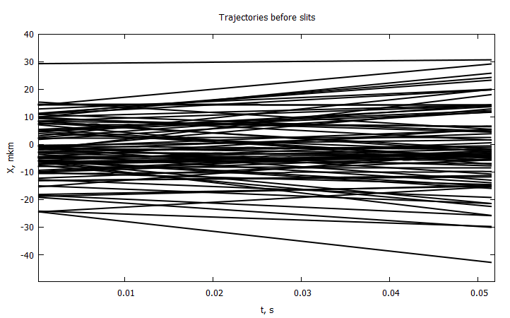

, , , , , . . . , .

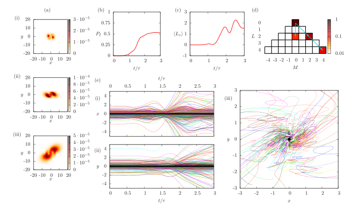
Y , , . X . .

" " ,

v_{x} (x, t) = \frac{1}{t - t_{1}} [x + \frac{- 1}{2 (α^{2} + β_{t}^{2})} (β_{t} I m (\frac{C (x, t)}{H (x, t)}) + α Re (\frac{C (x, t)}{H (x, t)}) - β_{t} γ_{x, t})]

$v_{x}(x, t)=\frac{1}{t-t_{1}}\left[x+\frac{-1}{2\left(\alpha^{2}+\beta_{t}^{2}\right)}\left(\beta_{t} I m\left(\frac{C(x, t)}{H(x, t)}\right)+\alpha \operatorname{Re}\left(\frac{C(x, t)}{H(x, t)}\right)-\beta_{t} \gamma_{x, t}\right)\right]$

18+

\begin{aligned} H (x, t) & = \int_{X_{A} - b}^{X_{A} + b} f (x, u, t) d u + \int_{X_{B} - b}^{X_{B} + b} f (x, u, t) d u \\ C (x, t) & = [f (x, u, t)]_{u = X_{A} - b}^{u = X_{A} + b} + [f (x, u, t)]_{u = X_{B} - b}^{u = X_{B} + b} \\ f (x, u, t) & = \exp [(α + i β_{t}) u^{2} + i γ_{x, t} u] \\ α & = - \frac{1}{4 σ_{0}^{2} (1 + {(\frac{ℏ t_{1}}{2 m σ_{0}^{2}})}^{2})} \\ β_{t} & = \frac{m}{2 ℏ} (\frac{1}{t - t_{1}} + \frac{1}{t_{1} (1 + {(\frac{2 m σ_{0}^{2}}{ℏ t_{1}})}^{2})}) \\ γ_{x, t} & = - \frac{m x}{ℏ (t - t_{1})} \end{aligned}

$\begin{aligned} H(x, t) &= \int_{X_{A}-b}^{X_{A}+b} f(x, u, t) d u+\int_{X_{B}-b}^{X_{B}+b} f(x, u, t) d u \\ C(x, t) &= [f(x, u, t)]_{u=X_{A}-b}^{u=X_{A}+b}+[f(x, u, t)]_{u=X_{B}-b}^{u=X_{B}+b} \\ f(x, u, t) &= \exp \left[\left(\alpha+i \beta_{t}\right) u^{2}+i \gamma_{x, t} u\right]\\ \alpha &= -\frac{1}{4 \sigma_{0}^{2}\left(1+\left(\frac{\hbar t_{1}}{2 m \sigma_{0}^{2}}\right)^{2}\right)} \\ \beta_{t} &= \frac{m}{2 \hbar}\left(\frac{1}{t-t_{1}}+\frac{1}{t_{1}\left(1+\left(\frac{2 m \sigma_{0}^{2}}{\hbar t_{1}}\right)^{2}\right)}\right) \\ \gamma_{x, t} &= -\frac{m x}{\hbar\left(t-t_{1}\right)} \end{aligned}$

function Uₓ(t, x)

    γ = -m*x / ( ħ*(t-tf1) )
    β = m/(2ħ) * ( 1/(t-tf1) + 1 / ( tf1*( 1 + (2m*σ₀^2 / (ħ*tf1) )^2 ) ) )
    α = -( 4σ₀^2 * ( 1 + ( ħ*tf1 / (2m*σ₀^2) )^2 ) )^-1

    f(x, u, t) = exp( ( α + im*β )*u^2 + im*γ*u )

    C = f(x, a2, t) - f(x, a1, t) + f(x, b2, t) - f(x, b1, t)
    H = trapez( u-> f(x, u, t) , a1, a2, 400) + trapez( u-> f(x, u, t) , b1, b2, 400)

    return 1/(t-tf1) * ( x - 0.5/(α^2 + β^2) * ( β*imag(C/H) + α*real(C/H) - β*γ ) )
end

init() = bitrand()[1] ? rand()*(b2 - b1) + b1 : rand()*(a2 - a1) + a1
myrng(a, b, N) = collect( range(a, stop = b, length = N ÷ 2) )

n = 1
xx = 0
ξ = 1e-5
while xx < Cron2[end]-Cron2[1]
    n+=1
    xx += (ξ*n)^2 
end
n

steps = [ (ξ*i)^2 for i in 1:n1 ]
Cronadapt = accumulate(+, steps, init = Cron2[1] )

function modelsolver(Np = 10, Nt = 100)

    #xo = [ init() for i = 1:Np ] # 
    xo = vcat( myrng(a2, a1, Np), myrng(b1, b2, Np) ) # 

    xpath = zeros(Nt, Np)
    xpath[1,:] = xo

    for i in 2:Nt, j in 1:Np
        xpath[i,j] = rk4(Uₓ, Cronadapt[i], xpath[i-1,j], steps[i] )
    end

    xpath
end

@time paths = modelsolver(20, n);

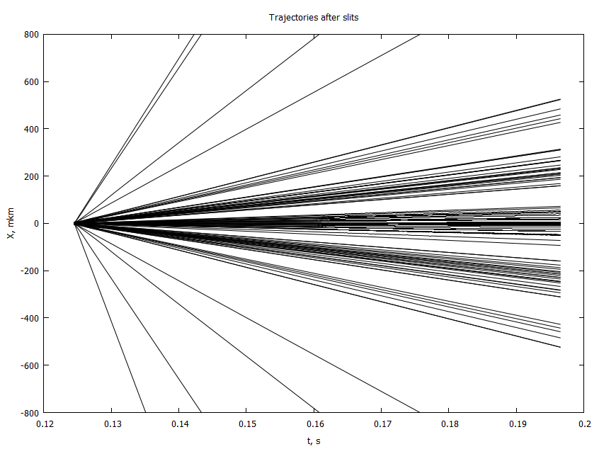
@gp "set title 'Trajectories after the slits'" xlab="t, s" ylab="X, mkm" "set yrange [-800:800]"
for i in 1:size(paths, 2)
    @gp :- Cronadapt 1e6paths[:,i] "with lines notit lw 1 lc rgb 'black'"
end

- 4 , . 2

, : , , .

. , ,

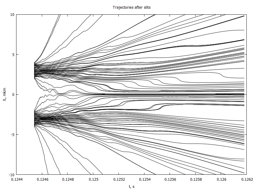
function yas(t, xo, yo, vo)

    cosϕ = xo / sqrt( xo^2 + yo^2 )
    sinϕ = yo / sqrt( xo^2 + yo^2 )
    atnx = -ħ*t / (2m*σ₀^2)
    sinatnx = atnx / sqrt( atnx^2 + 1)
    cosatnx =    1 / sqrt( atnx^2 + 1)
    #cosϕt = cosϕ * cosatnx - sinϕ * sinatnx
    sinϕt = sinϕ*cosatnx + cosϕ*sinatnx

    σ₀t = sqrt( σ₀^2 + ( ħ*t / (2*m*σ₀) )^2 )

    vo*t + sqrt(xo^2 + yo^2) * σ₀t/σ₀ * sinϕt
end

function modelsolver2(Np = 10)

    Nt = length(Cronadapt)
    xo = [ init() for i = 1:Np ]
    #xo = vcat( myrng(a2, a1, Np), myrng(b1, b2, Np) )

    xcoord = copy(xo)
    ycoord = zeros(Np)

    for i in 2:Nt, j in 1:Np
        xcoord[j] = rk4(Uₓ, Cronadapt[i], xcoord[j], steps[i] )
    end

    for (i, x) in enumerate(xo)

        y0 = randn()*yh
        v0 = 0 #randn()*σv*1e-4

        ycoord[i] = yas(Cronadapt[end], x, y0, v0)
    end

    xcoord, ycoord
end

@time X, Y = modelsolver2(100);

@gp "set title 'Impacts on the screen'" xlab="X, mm" ylab="Y, mm"# "set xrange [-1:1]"
@gp :- 1000X 1000Y "with points notit pt 7 ps 0.5 lc rgb 'black'"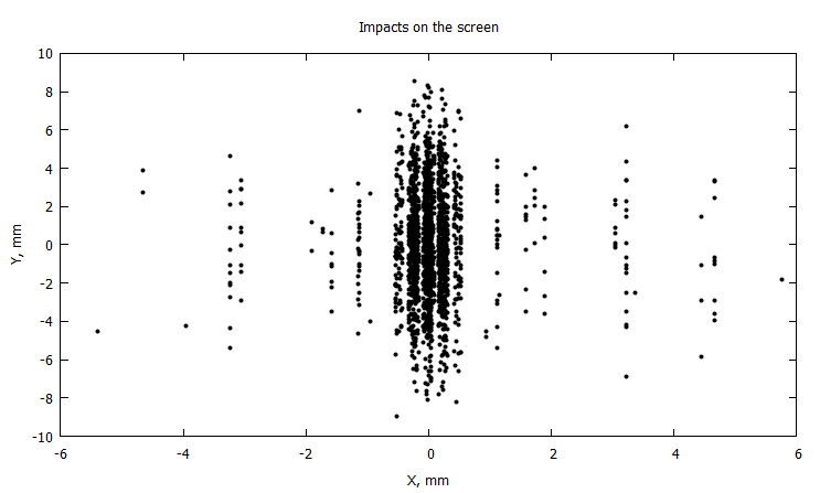

, , . , ,

, , , , , — , .

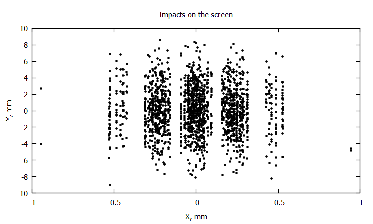
Obszöne Anwendung

More articles: