Guten Tag, habraledi und habragentelmen! In diesem Artikel werden wir unseren Einstieg in die Statistik mit Python fortsetzen. Wenn jemand den Beginn des Tauchgangs verpasst hat, ist hier ein Link zum ersten Teil . Wenn nicht, empfehle ich dennoch, Sarah Boslafs offenes Buch "Statistik für alle" immer zur Hand zu haben. Ich empfehle außerdem, Notepad auszuführen, um mit Code und Grafiken zu experimentieren.
Wie Andrew Lang sagte: „ Statistiken sind für einen Politiker wie eine Straßenlaterne für einen betrunkenen Mist: eher eine Requisite als eine Beleuchtung. “ Dasselbe gilt für diesen Artikel für Neulinge. Es ist unwahrscheinlich, dass Sie hier viel neues Wissen lernen, aber ich hoffe, dieser Artikel hilft Ihnen zu verstehen, wie Sie Python verwenden, um das Selbststudium von Statistiken zu erleichtern.
Warum neue Zuordnungen erfinden?
Stellen Sie sich vor ... bevor wir uns etwas vorstellen, lassen Sie uns noch einmal alle notwendigen Importe durchführen:
import numpy as np
from scipy import stats
import matplotlib.pyplot as plt
import seaborn as sns
from pylab import rcParams
sns.set()
rcParams['figure.figsize'] = 10, 6
%config InlineBackend.figure_format = 'svg'
np.random.seed(42)
, , . , , - , . 1000 100- , . :
gen_pop = np.trunc(stats.norm.rvs(loc=80, scale=5, size=1000))
gen_pop[gen_pop>100]=100
print(f'mean = {gen_pop.mean():.3}')
print(f'std = {gen_pop.std():.3}')
mean = 79.5
std = 4.95
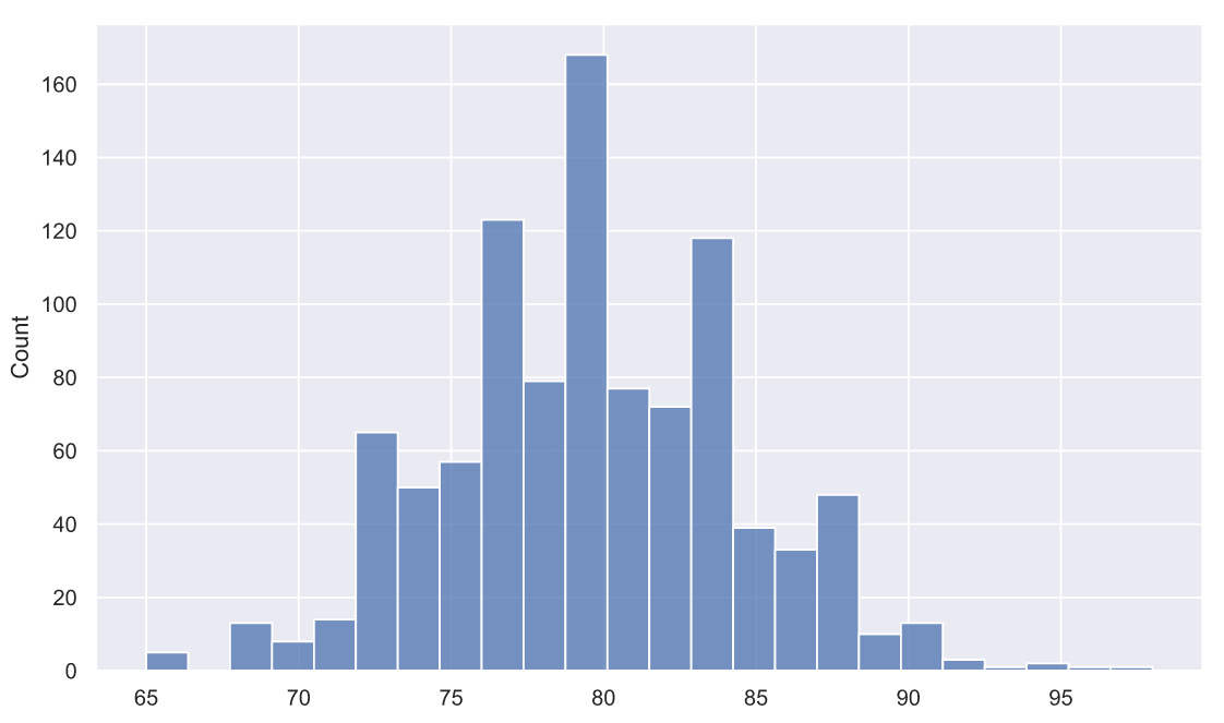
, , . 80 5 . , , , , , - .
, . , - . , - , ? - . , 10 , :
![[89, 99, 93, 84, 79, 61, 82, 81, 87, 82]](https://habrastorage.org/getpro/habr/upload_files/111/47c/b45/11147cb4509f3d49e1c731d87a8b657b.svg)
Z- :

 - ,
- , 
 ,
,  - . :
- . :
sample = np.array([89,99,93,84,79,61,82,81,87,82])
sample.mean()
83.7
Z-:
z = 10**0.5*(sample.mean()-80)/5
z
2.340085468524603
p-value:
1 - (stats.norm.cdf(z) - stats.norm.cdf(-z))
0.019279327322753836
, , : Z- 0 2 , .. 10 , , , 0.02. , 10 , ""  , , 10 "" 83.7 2%. , , , , . .
- 10 , , :
sample.std(ddof=1)
10.055954565441423
ddof std
 , ,
, ,  , . :
, . :

, ,  . -
. - 
 ,
, 
 .
. 
 ? ,
? , 
 -
-  ,
,  .
.  , - .
, - .
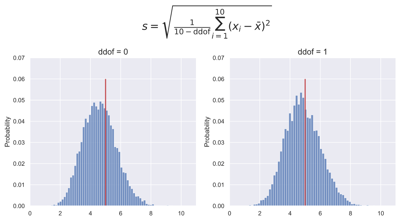
, std() NumPy ddof, 0, std() , , ddof=1. . , 10000 10  , , ddof=0 . ddof=1 , - , ddof=0:
fig, ax = plt.subplots(nrows=1, ncols=2, figsize = (12, 5))
for i in [0, 1]:
deviations = np.std(stats.norm.rvs(80, 5, (10000, 10)), axis=1, ddof=i)
sns.histplot(x=deviations ,stat='probability', ax=ax[i])
ax[i].vlines(5, 0, 0.06, color='r', lw=2)
ax[i].set_title('ddof = ' + str(i), fontsize = 15)
ax[i].set_ylim(0, 0.07)
ax[i].set_xlim(0, 11)
fig.suptitle(r'$s={\sqrt {{\frac {1}{10 - \mathrm{ddof}}}\sum _{i=1}^{10}\left(x_{i}-{\bar {x}}\right)^{2}}}$',
fontsize = 20, y=1.15);
, Z-? , - , . 5000 10 ,  :
:
deviations = np.std(stats.norm.rvs(80, 5, (5000, 10)), axis=1, ddof=1)
sns.histplot(x=deviations ,stat='probability');

, , 10- . . , , 10 2%, , ( ) 10 0. , , : 10- , .
, , , : - , - , . , ""  , Z- p-value 10- :
z = 10**0.5*(sample.mean()-80)/10
p = 1 - (stats.norm.cdf(z) - stats.norm.cdf(-z))
print(f'z = {z:.3}')
print(f'p-value = {p:.4}')
z = 1.17
p-value = 0.242
,  , , , .. ,
  , . 2%, 25%. , -
 .
.
, ? ! , : (, , - )

T-, Z- ,  ,
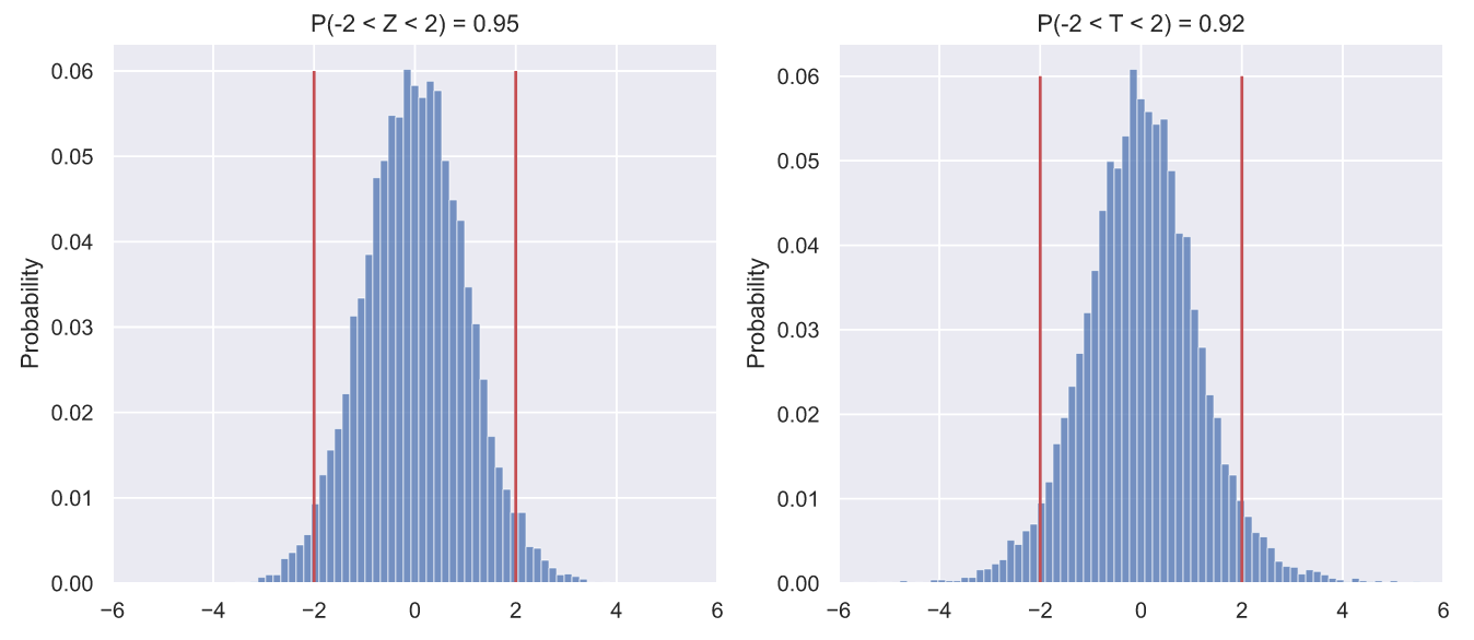
,  . 10000
  , Z- T-, :
fig, ax = plt.subplots(nrows=1, ncols=2, figsize = (12, 5))
N = 10000
samples = stats.norm.rvs(80, 5, (N, 10))
statistics = [lambda x: 10**0.5*(np.mean(x, axis=1) - 80)/5,
lambda x: 10**0.5*(np.mean(x, axis=1) - 80)/np.std(x, axis=1, ddof=1)]
title = 'ZT'
bins = np.linspace(-6, 6, 80, endpoint=True)
for i in range(2):
values = statistics[i](samples)
sns.histplot(x=values ,stat='probability', bins=bins, ax=ax[i])
p = values[(values > -2)&(values < 2)].size/N
ax[i].set_title('P(-2 < {} < 2) = {:.3}'.format(title[i], p))
ax[i].set_xlim(-6, 6)
ax[i].vlines([-2, 2], 0, 0.06, color='r');
- :
import matplotlib.animation as animation
fig, axes = plt.subplots(nrows=1, ncols=2, figsize = (18, 8))
def animate(i):
for ax in axes:
ax.clear()
N = 10000
samples = stats.norm.rvs(80, 5, (N, 10))
statistics = [lambda x: 10**0.5*(np.mean(x, axis=1) - 80)/5,
lambda x: 10**0.5*(np.mean(x, axis=1) - 80)/np.std(x, axis=1, ddof=1)]
title = 'ZT'
bins = np.linspace(-6, 6, 80, endpoint=True)
for j in range(2):
values = statistics[j](samples)
sns.histplot(x=values ,stat='probability', bins=bins, ax=axes[j])
p = values[(values > -2)&(values < 2)].size/N
axes[j].set_title(r'$P(-2\sigma < {} < 2\sigma) = {:.3}$'.format(title[j], p))
axes[j].set_xlim(-6, 6)
axes[j].set_ylim(0, 0.07)
axes[j].vlines([-2, 2], 0, 0.06, color='r')
return axes
dist_animation = animation.FuncAnimation(fig,
animate,
frames=np.arange(7),
interval = 200,
repeat = False)
dist_animation.save('statistics_dist.gif',
writer='imagemagick',
fps=1)
, , . ? -, , . , , ? , , 
![[-2 \ Sigma; 2 \ sigma]](https://habrastorage.org/getpro/habr/upload_files/f0d/a1c/cfd/f0da1ccfdb352631a44937d502801011.svg) 95.5% . Z- , T- , 92-93% . , , - , :
95.5% . Z- , T- , 92-93% . , , - , :
statistics = [lambda x: 10**0.5*(np.mean(x, axis=1) - 80)/5,
lambda x: 10**0.5*(np.mean(x, axis=1) - 80)/np.std(x, axis=1, ddof=1)]
quantity = 50
N=10000
result = []
for i in range(quantity):
samples = stats.norm.rvs(80, 5, (N, 10))
Z = statistics[0](samples)
p_z = Z[(Z > -2)&((Z < 2))].size/N
T = statistics[1](samples)
p_t = T[(T > -2)&((T < 2))].size/N
result.append([p_z, p_t])
result = np.array(result)
fig, ax = plt.subplots()
line1, line2 = ax.plot(np.arange(quantity), result)
ax.legend([line1, line2],
[r'$P(-2\sigma < {} < 2\sigma)$'.format(i) for i in 'ZT'])
ax.hlines(result.mean(axis=0), 0, 50, color='0.6');
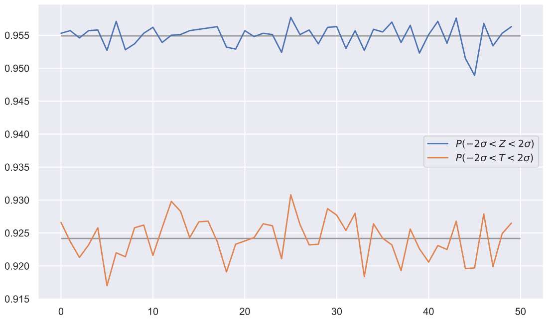
50 . , , , , . ? , ! Z- T- , . , T- ? , - . , , - , , , . , . , - , , 
 .
.
Z-,  ,
,  - . 10000
  10 , :
# ,
# svg png:
#%config InlineBackend.figure_format = 'png'
N = 10000
samples = stats.norm.rvs(80, 5, (N, 10))
means = samples.mean(axis=1)
deviations = samples.std(ddof=1, axis=1)
T = statistics[1](samples)
P = (T > -2)&((T < 2))
fig, ax = plt.subplots()
ax.scatter(means[P], deviations[P], c='b', alpha=0.7,
label=r'$\left | T \right | < 2\sigma$')
ax.scatter(means[~P], deviations[~P], c='r', alpha=0.7,
label=r'$\left | T \right | > 2\sigma$')
mean_x = np.linspace(75, 85, 300)
s = np.abs(10**0.5*(mean_x - 80)/2)
ax.plot(mean_x, s, color='k',
label=r'$\frac{\sqrt{n}(\bar{x}-\mu)}{2}$')
ax.legend(loc = 'upper right', fontsize = 15)
ax.set_title(' \n ',
fontsize=15)
ax.set_xlabel(r' ($\bar{x}$)',
fontsize=15)
ax.set_ylabel(r' ($s$)',
fontsize=15);
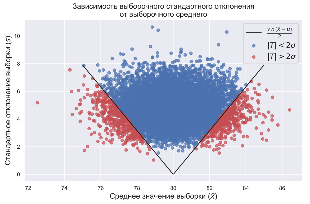
, . , , 
 , .. . , ,
  ,
, 
 . , ( ) , :

,  , .. , , ,
  ,
,  :
:

, ![[-2\sigma; 2\sigma]](https://habrastorage.org/getpro/habr/upload_files/bea/828/453/bea828453e4b32cb920e5d40a188262d.svg) , , 92,5% .
, , 92,5% .
? , . , ( ) 100- . , , ( ). 10- 82- , 2- . , , .  , , ..
  ? Z-:
? Z-:

 p-value:
z = 10**0.5*(82-80)/2
p = 1 - (stats.norm.cdf(z) - stats.norm.cdf(-z))
print(f'p-value = {p:.2}')
p-value = 0.0016
10 82- 2%.  . ,
. ,  , , , .
, , , . (  ) (
) (  ).
).
10 . 82 , , , 9- . ? :
z = 10**0.5*(82-80)/9
p = 1 - (stats.norm.cdf(z) - stats.norm.cdf(-z))
print(f'p-value = {p:.2}')
p-value = 0.48
10 

 . , , - .
, , . :
import matplotlib.animation as animation
fig, ax = plt.subplots(figsize = (15, 9))
def animate(i):
ax.clear()
N = 10000
samples = stats.norm.rvs(80, 5, (N, i))
means = samples.mean(axis=1)
deviations = samples.std(ddof=1, axis=1)
T = i**0.5*(np.mean(samples, axis=1) - 80)/np.std(samples, axis=1, ddof=1)
P = (T > -2)&((T < 2))
prob = T[P].size/N
ax.set_title(r' $s$ $\bar{x}$ $n = $' + r'${}$'.format(i),
fontsize = 20)
ax.scatter(means[P], deviations[P], c='b', alpha=0.7,
label=r'$\left | T \right | < 2\sigma$')
ax.scatter(means[~P], deviations[~P], c='r', alpha=0.7,
label=r'$\left | T \right | > 2\sigma$')
mean_x = np.linspace(75, 85, 300)
s = np.abs(i**0.5*(mean_x - 80)/2)
ax.plot(mean_x, s, color='k',
label=r'$\frac{\sqrt{n}(\bar{x}-\mu)}{2}$')
ax.legend(loc = 'upper right', fontsize = 15)
ax.set_xlim(70, 90)
ax.set_ylim(0, 10)
ax.set_xlabel(r' ($\bar{x}$)',
fontsize='20')
ax.set_ylabel(r' ($s$)',
fontsize='20')
return ax
dist_animation = animation.FuncAnimation(fig,
animate,
frames=np.arange(5, 21),
interval = 200,
repeat = False)
dist_animation.save('sigma_rel.gif',
writer='imagemagick',
fps=3)

, 


 , .
, .  Z-,
Z-,  .
.
! , ? - , , . , , 10- :
![[89,99,93,84,79,61,82,81,87,82]](https://habrastorage.org/getpro/habr/upload_files/e5d/05a/011/e5d05a011425a07da6167192fdea7c18.svg)
 ,
,  , , , , ,
  . Z-, T-, Z- ,
 . , -
. , -  ,
,  - ?
- ?  ?: ,
?: ,  ,
,  ,
, 
 ?
?
, . , - . ,  , , , 10 , 10 . ,
  . , - , .
:  ,
,  ,
, 
 . , ,
. , , 
 :
:
N = 10000
sigma = np.linspace(5, 20, 151)
prob = []
for i in sigma:
p = []
for j in range(10):
samples = stats.norm.rvs(80, i, (N, 10))
means = samples.mean(axis=1)
deviations = samples.std(ddof=1, axis=1)
p_m = means[(means >= 83) & (means <= 84)].size/N
p_d = deviations[(deviations >= 9.5) & (deviations <= 10.5)].size/N
p.append(p_m*p_d)
prob.append(sum(p)/len(p))
prob = np.array(prob)
fig, ax = plt.subplots()
ax.plot(sigma, prob)
ax.set_xlabel(r' ($\sigma$)',
fontsize=20)
ax.set_ylabel('',
fontsize=20);
,  . , ,
. , ,  ,
,  . - , , , , . .
T-?
, - - . 1% , - . , , . , - -. ?
- ! , - , "" t-. , , , . , , 1943 , 50% . , - .
, "" . , ( !) , "" , :

t-, . , , "", , , , , - . " ", "t-" , .
:

" " .  , ..
, ..  ,
,  , .. , . - , :

, :
import matplotlib.animation as animation
fig, ax = plt.subplots(figsize = (15, 9))
def animate(i):
ax.clear()
N = 15000
x = np.linspace(-5, 5, 100)
ax.plot(x, stats.norm.pdf(x, 0, 1), color='r')
samples = stats.norm.rvs(0, 1, (N, i))
t = samples[:, 0]/np.sqrt(np.mean(samples[:, 1:]**2, axis=1))
t = t[(t>-5)&(t<5)]
sns.histplot(x=t, bins=np.linspace(-5, 5, 100), stat='density', ax=ax)
ax.set_title(r' $t(n)$ n = ' + str(i), fontsize = 20)
ax.set_xlim(-5, 5)
ax.set_ylim(0, 0.5)
return ax
dist_animation = animation.FuncAnimation(fig,
animate,
frames=np.arange(2, 21),
interval = 200,
repeat = False)
dist_animation.save('t_rel_of_df.gif',
writer='imagemagick',
fps=3)
,  , , ,
, , ,  . , , :

SciPy:
import matplotlib.animation as animation
fig, ax = plt.subplots(figsize = (15, 9))
def animate(i):
ax.clear()
N = 15000
x = np.linspace(-5, 5, 100)
ax.plot(x, stats.norm.pdf(x, 0, 1), color='r')
ax.plot(x, stats.t.pdf(x, df=i))
ax.set_title(r' $t(n)$ n = ' + str(i), fontsize = 20)
ax.set_xlim(-5, 5)
ax.set_ylim(0, 0.45)
return ax
dist_animation = animation.FuncAnimation(fig,
animate,
frames=np.arange(2, 21),
interval = 200,
repeat = False)
dist_animation.save('t_pdf_rel_of_df.gif',
writer='imagemagick',
fps=3)

,  ( df ) . - , ,
  , .
, .
t-
t- SciPy :
sample = np.array([89,99,93,84,79,61,82,81,87,82])
stats.ttest_1samp(sample, 80)
Ttest_1sampResult(statistic=1.163532240174695, pvalue=0.2745321678073461)
:
T = 9**0.5*(sample.mean() -80)/sample.std()
T
1.163532240174695
,  ,
,  ,
,  . , 1 , , , . :
T = 10**0.5*(sample.mean() -80)/sample.std(ddof=1)
T
1.1635322401746953
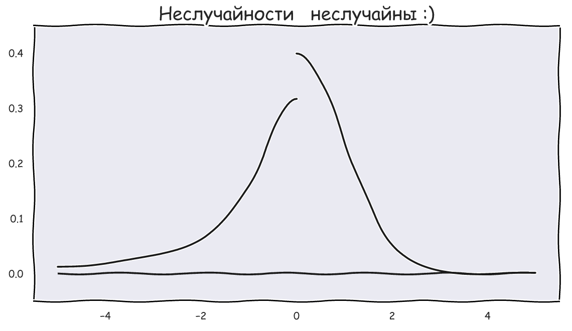
, t- , p-value? , - , p-value Z-, t-:
t = stats.t(df=9)
fig, ax = plt.subplots()
x = np.linspace(t.ppf(0.001), t.ppf(0.999), 300)
ax.plot(x, t.pdf(x))
ax.hlines(0, x.min(), x.max(), lw=1, color='k')
ax.vlines([-T, T], 0, 0.4, color='g', lw=2)
x_le_T, x_ge_T = x[x<-T], x[x>T]
ax.fill_between(x_le_T, t.pdf(x_le_T), np.zeros(len(x_le_T)), alpha=0.3, color='b')
ax.fill_between(x_ge_T, t.pdf(x_ge_T), np.zeros(len(x_ge_T)), alpha=0.3, color='b')
p = 1 - (t.cdf(T) - t.cdf(-T))
ax.set_title(r'$P(\left | T \right | \geqslant {:.3}) = {:.3}$'.format(T, p));

, p-value 27%, .. , - ,  , p-value , 5 . , , - ,
  , 0.95:

SciPy, interval loc () scale () :
sample_loc = sample.mean()
sample_scale = sample.std(ddof=1)/10**0.5
ci = stats.t.interval(0.95, df=9, loc=sample_loc, scale=sample_scale)
ci
(76.50640345566619, 90.89359654433382)
,  , ,
, , 
![[76,5; 90,9]](https://habrastorage.org/getpro/habr/upload_files/271/4c8/21d/2714c821d6a7a520116d1a2df7c3059c.svg) . , ,
. , ,  , .
, .
, , , ( ). , , t- , t- , t- .
Natürlich möchte ich am Ende ein GIF einfügen, aber ich möchte mit dem Satz von Herbert Spencer enden: " Das größte Ziel der Bildung ist nicht Wissen, sondern Handeln ". Starten Sie also Ihre Anakondas und ergreifen Sie Maßnahmen ! Dies gilt insbesondere für Autodidakten wie mich.
Ich drücke F5 und freue mich auf Ihre Kommentare!