🧥 🖋️ 👇🏿 Matrix-Rematrix ⚫️ 🥨 👒

Die Arbeit eines neuronalen Netzwerks basiert auf Matrixmanipulation. Für das Training werden verschiedene Methoden verwendet, von denen viele aus der Gradientenabstiegsmethode hervorgegangen sind, bei der es erforderlich ist, mit Matrizen umgehen zu können, um Gradienten (Ableitungen in Bezug auf Matrizen) zu berechnen. Wenn Sie unter die Haube eines neuronalen Netzwerks schauen, sehen Sie Matrizenketten, die oft einschüchternd wirken. Einfach ausgedrückt: „Die Matrix wartet auf uns alle“. Es ist Zeit, sich besser kennenzulernen.

Dazu führen wir folgende Schritte aus:

: , , ;
;
.

NumPy . , , , , . , , , - , , , . , - : , .

-

- , , , . , , , Google TensorFlow.

, , , , , $a_ {i}$ , i = 0, 1, 2, ..., n-1 ; - .

import numpy as np #   numpy
a=np.array([1,2,5])
a.ndim #  ,   = 1
a.shape #      (3,)
a.shape[0] #      = 3

$a_ {i} \ cdot b_ {i} = a_ {0} \ cdot b_ {0} + a_ {1} \ cdot b_ {1} + a_ {2} \ cdot b_ {2}$ . , , 0 2 .

b=np.array([3,4,7])
np.dot(a,b) #   = 46
a*b #   array([ 3,  8, 35])
np.sum(a*b) # = 46

( ) - , $A_ {i, j}$ . , $A_ {0, 2}$ - 0- 2- . , .

A=np.array([[ 1,  2,  3],
            [ 2,  4,  6]])
A # array([[1, 2, 3],
  #        [2, 4, 6]])
A[0, 2] #    ,    = 3
A.shape # (2, 3)   2 , 3

EIN C = AB , $C_ {i, k} = A_ {i, j} B_ {j, k}$ . , EIN ( EIN )

B=np.array([[7, 8, 1, 3],
            [5, 4, 2, 7],
            [3, 6, 9, 4]])
A.shape[1] == B.shape[0] # true
A.shape[1], B.shape[0] # (3, 3) 
A.shape, B.shape # ((2, 3), (3, 4))
C = np.dot(A, B)
C # array([[26, 34, 32, 29],
  #        [52, 68, 64, 58]]); 
  #  , C[0,1]=A[0,0]B[0,1]+ A[0,1]B[1,1]+A[0,2]B[2,1]=1*8+2*4+3*6=34
C.shape # (2, 4)

, :

np.dot(B, A) # ValueError: shapes (3,4) and (2,3) not aligned: 4 (dim 1) != 2 (dim 0)

EIN , .

, . , $a_ {i, 0}$ $b_ {j, 0}$ . $D_ {i, j} = a_ {i, 0} b_ {j, 0}$ . , , , $b_ {j, 0} = (bT) _ {0, j}$ , - ( NumPy). $D = a \ cdot bT$ . , $DT = (a \ cdot bT) .T = (bTT) \ cdot aT = b \ cdot aT$ .

a = np.reshape(a, (3,1)) #   ,  a.shape = (3,)  (3,1),
b = np.reshape(b, (3,1)) #  ,  
D = np.dot(a,b.T)
D # array([[ 3,  4,  7],
  #        [ 6,  8, 14],
  #        [15, 20, 35]])

, . , .

, , . (cost function). , . . , (learning rate), , (epoch). , . (), . . , , , .

, ( , ).

- (samples) . . , (), ( ) - (samples), - (features).

, ( ). (, …) , , . , .

!

, , . , “ ” . , , . , , . , , , .

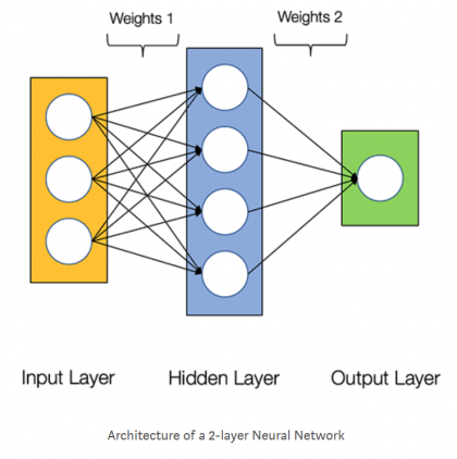
, 10 . , (10, 3). “ ”, . , . , :

, , 0 50 ;

X=np.random.randint(0, 50, (10, 3))

0 1;

X=np.random.rand(10, 3)

$\ mu = 2$ $\ sigma ^ 2 = 16$ . , , $N (\ mu, \ sigma ^ 2)$ ;

X=4*np.random.randn(10, 3) + 2

$\ mu = 0$ $\ sigma = 1$ , .

, (10, 3) $W ^ {(1)}$ , . , , . , , , $W ^ {(1)}$ (3, 4) . , $(10, 3) (3, 4) \ Rightarrow (10, 4)$ . , $X \ cdot W ^ {(1)}$ (10.4) , - - , . . , EIN (m, n) ( , ) $a_ {i, j}$ , f (A) , $f (a_ {i, j})$ ; , , $a_ {1,2} \ Rightarrow f (a_ {1,2})$ , . , $W ^ {(2)}$ , (4, 1) . , $(10, 3) (3, 4) (4, 1) \ Rightarrow (10, 1)$ . , $\hat{Y}$ 10- (samples) . :

$\hat{Y}=X\cdot W^{(1)}\cdot W^{(2)}, \quad\quad \hat{Y}_{i,0}=X_{i,j} W_{j,k}^{(1)} W_{k,0}^{(2)}.$

, . (bias).

. : , , , .

X=np.random.randint(0, 50, (10, 3))
w1=2*np.random.rand(3,4)-1 #       -1  +1
w2=2*np.random.rand(4,1)-1
Y=np.dot(np.dot(x,w1),w2) #   
Y.shape # (10, 1)
Y.T.shape # (1, 10)
(np.dot(Y.T,Y)).shape # (1, 1), ,

. -1 +1, “” ( ).

. f_1 “ ”, - .

$\hat{Y}_{i,0}=f_2(f_1(X_{i,j} W_{j,k}^{(1)})W_{k,0}^{(2)}),$ $\hat{Y}=f_2(f_1(X \cdot W^{(1)})\cdot W^{(2)}).$

, .

$\triangle=\sum_i(Y_{i,0}-\hat{Y}_{i,0})^2=\sum_i\widetilde{Y}_{i,0}^2=(\widetilde{Y}.T)_{0,i}\widetilde{Y}_{i,0}=(\widetilde{Y}.T)\cdot\widetilde{Y},$

(X,Y) - , $\widetilde{Y}_{i,0}=Y_{i,0}-\hat{Y}_{i,0}$ . , $(\widetilde{Y}.T)_{0,i}=\widetilde{Y}_{i,0}$ .

, . .

. - . , . , .

- , . f(x) $f^{'}(x_0)=0$ , “ ” - . , , . , , . : - , , - . (, 16 ), , . . , $f^{'}(W)<0$ , , , $f^{'}(W)>0$ , . , .

$W\Rightarrow W+\mu\cdot\delta W=W-\mu\cdot\frac{\partial \triangle}{\partial W},$

$W_{i,j}\Rightarrow W_{i,j}+\mu\cdot\delta W_{i,j}=W_{i,j}-\mu\cdot\frac{\partial \triangle}{\partial W_{i,j}},$

$\mu$ - (learning rate). , . . - , , . , - .

.

$\frac{\partial a_{m, n}}{\partial a_{i,j}}=\delta_{m,i}\delta_{n,j},$

$\delta_{i,j}$ - , , i=j . , $\delta_{1,1}=1$ , $\delta_{2,1}=0$ . : .

$\frac{\partial \triangle}{\partial W_{m,n}}=-2\sum_i(Y_{i,0}-\hat{Y}_{i,0})\frac{\partial \hat{Y}_{i,0}}{\partial W_{m,n}}=-2\widetilde{Y}_{i,0}\frac{\partial \hat{Y}_{i,0}}{\partial W_{m,n}},$

, , $\widetilde{Y}_{i,0}=Y_{i,0}-\hat{Y}_{i,0}$ , .

. . , , .

, $\hat{Y}_{i,0}=X_{i,j} W_{j,k}^{(1)} W_{k,0}^{(2)}$ ,

$\frac{\partial \triangle}{\partial W_{m,0}^{(2)}}=-2\widetilde{Y}_{i,0}\frac{\partial \hat{Y}_{i,0}}{\partial W_{m,0}^{(2)}}=-2\widetilde{Y}_{i,0}X_{i,j} W_{j,k}^{(1)}\delta_{k,m}=-2\widetilde{Y}_{i,0}X_{i,j} W_{j,m}^{(1)}=-2\widetilde{Y}_{i,0}(X\cdot W^{(1)})_{i,m}$

, $A_{i,m}=(A.T)_{m.i}$ . , :

$\delta W_{m,0}^{(2)}=-\frac{\partial \triangle}{\partial W_{m,0}^{(2)}}=2((X\cdot W^{(1)}).T)_{m,i}\widetilde{Y}_{i,0},$

$\delta W^{(2)}=2((X\cdot W^{(1)}).T)\cdot \widetilde{Y}.$

, , , $\delta W^{(2)}$ . $X\cdot W^{(1)}$ (10,3)(3,4)=(10,4) , - (4,10) . $\widetilde{Y}$ $\hat{Y}$ - (10,1) . , $\delta W^{(2)}$ (4,10)(10,1)=(4,1) , .

deltaW2=2*np.dot(np.dot(X,w1).T,Y)
deltaW2.shape # (4,1)

$W^{(1)}$ .

$\frac{\partial \triangle}{\partial W_{m,n}^{(1)}}=-2\widetilde{Y}_{i,0}\frac{\partial \hat{Y}_{i,0}}{\partial W_{m,n}^{(1)}}=-2\widetilde{Y}_{i,0}X_{i,j} \delta_{j,m}\delta_{k,n}W_{k,0}^{(2)}=-2\widetilde{Y}_{i,0}X_{i,m} W_{n,0}^{(2)}=-2(X.T)_{m,i}\widetilde{Y}_{i,0}(W^{(2)}.T)_{0,n},$ $\delta W^{(1)}=2(X.T)\cdot \widetilde{Y}\cdot (W^{(2)}.T).$

, “ ”, “ ” - . , , . : “” ( ), , .

$\delta W^{(1)}$ : (3,10)(10,1)(1,4)=(3,4) .

. ,, , , . . , . , . , , : z=f(y(x)) , $z_x^{'}=f_y^{'}y_x^{'}$ .

$\hat{Y}_{i,0}=f_2(f_1(X_{i,j} W_{j,k}^{(1)})W_{k,0}^{(2)})\quad\Rightarrow\quad \hat{Y}_{i,0}=f_2(C_{i,0}),$

$C_{i,0}=B_{i,k}W_{k,0}^{(2)}, \quad\quad B_{i,k}=f_1(A_{i,k}), \quad\quad A_{i,k}=X_{i,j} W_{j,k}^{(1)}.$

W_2 , . ,

$\delta W_{m,0}^{(2)}=2\widetilde{Y}_{i,0}\frac{\partial \hat{Y}_{i,0}}{\partial W_{m,0}^{(2)}}=2\widetilde{Y}_{i,0}\frac{\partial f_2(C_{i,0})}{\partial C_{\mu,0}}\frac{\partial C_{\mu,0}}{\partial W_{m,0}^{(2)}}=2\widetilde{Y}_{i,0}f_2^{'}(C_{i,0})\delta_{i,\mu}B_{\mu,k}\delta_{k,m}=2\widetilde{Y}_{i,0}f_2^{'}(C_{i,0})B_{i,m}.$

$\frac{\partial f_2(C_{i,0})}{\partial C_{\mu,0}}=f_2^{'}(C_{i,0})\delta_{i,\mu}, \quad\quad \frac{\partial C_{\mu,0}}{\partial W_{m,0}^{(2)}}=B_{\mu,k}\frac{\partial W_{k,0}^{(2)}}{\partial W_{m,0}^{(2)}}=B_{\mu,k}\delta_{k,m}.$

, - . : $B_{i,m}=(B.T)_{m,i}$ , $f_1(A_{i,m})=(f_1(A).T)_{m,i}$ . ,

$\delta W_{m,0}^{(2)}=2(B.T)_{m,i}\widetilde{Y}_{i,0}f_2^{'}(C_{i,0}) \Rightarrow \delta W^{(2)}=2(B.T)\cdot(\widetilde{Y}*f_2^{'}(C))$

“*” . , , , a*b , ; , $a_{1,2}b_{1,2}$ .

. f_1(x)=x^2 f_2(x)=x^3 . , , . NumPy .

def f1(x): #  
    return np.power(x,2)
def graf1(x): # 
    return 2*x
def f2(x): #  
    return np.power(x,3)
def gradf2(x): # 
    return 3*np.power(x,2)

A=np.dot(X,w1) #   
B=f1(A)        #   
C=np.dot(B,w2) #    
Y=f2() #   
deltaW2=2*np.dot(B.T, Y*gradf2(C))
deltaW2.shape # (4,1)

$W^{(1)}$ , . - .

$\delta W_{m,n}^{(1)}=2\widetilde{Y}_{i,0}\frac{\partial \hat{Y}_{i,0}}{\partial W_{m,n}^{(1)}}=2\widetilde{Y}_{i,0}\frac{\partial f_2(C_{i,0})}{\partial C_{\mu,\nu}}\frac{\partial C_{\mu,\nu}}{\partial B_{l,s}}\frac{\partial B_{l,s}}{\partial W_{m,n}^{(1)}},$

$C_{\mu,\nu}=B_{\mu,k}W_{k,\nu}^{(2)}$ . :

$\frac{\partial f_2(C_{i,0})}{\partial C_{\mu,\nu}}=f_2^{'}(C_{i,0})\delta_{i,\mu}\delta_{0,\nu},\quad\quad \frac{\partial C_{\mu,\nu}}{\partial B_{l,s}}=\delta_{\mu,l}\delta_{k,s}W_{k,\nu}^{(2)},\quad\quad$ $\frac{\partial B_{l,s}}{\partial W_{m,n}^{(1)}}=\frac{\partial B_{l,s}}{\partial A_{r,e}}\frac{\partial A_{r,e}}{\partial W_{m,n}^{(1)}}=f_1^{'}(A_{l,s})\delta_{l,r}\delta_{s,e}\delta_{j,m}\delta_{e,n}X_{r,j}=f_1^{'}(A_{l,s})\delta_{l,r}\delta_{s,n}X_{r,m}.$

$\ delta W_ {m, n} ^ {(1)} = 2 \ widetilde {Y} _ {i, 0} f_2 ^ {'} (C_ {i, 0}) \ delta_ {i, \ mu} \ delta_ {0, \ nu} \ delta _ {\ mu, l} \ delta_ {k, s} W_ {k, \ nu} ^ {(2)} f_1 ^ {'} (A_ {l, s}) \ delta_ {s, n} \ delta_ {l, r} X_ {r, m} = 2 \ widetilde {Y} _ {i, 0} f_2 ^ {'} (C_ {i, 0}) W_ {n, 0} ^ {(2)} f_1 ^ {'} (A_ {i, n}) X_ {i, m},$

$\ delta_ {i, \ mu} \ delta_ {0, \ nu} \ delta _ {\ mu, l} \ delta_ {k, s} \ delta_ {s, n} \ delta_ {l, r} = \ delta_ { i, l} \ delta_ {i, r} \ delta_ {k, n} \ delta_ {s, n}.$

, $\ delta_ {0, \ nu} W_ {k, \ nu} ^ {(2)} = W_ {k, 0} ^ {(2)}$ , , “”, l, r, k, s .

“” ,

$\ delta W_ {m, n} ^ {(1)} = 2 (XT) _ {m, i} \ widetilde {Y} _ {i, 0} f_2 ^ {'} (C_ {i, 0}) ( W ^ {(2)}. T) _ {0, n} f_1 ^ {'} (A_ {i, n}),$ $\ delta W ^ {(1)} = 2 (XT) \ cdot [[(\ widetilde {Y} * f_2 ^ {'} (C)) \ cdot (W ^ {(2)}. T)] * f_1 ^ {'} (A)].$

, $D_ {i, o} = \ widetilde {Y} _ {i, 0} f_2 ^ {'} (C_ {i, 0}) \ Rightarrow \ widetilde {Y} * f_2 ^ {'} (C)$ , $F_ {i, n} = D_ {io} (W ^ {(2)}. T) _ {0, n}$ , $F_ {i, n} f_1 ^ {'} (A_ {i, n}) \ Rechtspfeil F * f_1 ^ {'} (A)$ .

deltaW1=2*np.dot(X.T, np.dot(Y*gradf2(C),w2.T)*gradf1(A))
deltaW1.shape # (3,4)

. .

“, - . -!” ? , , , . , . - , , . ! , , - . , , .

, . James Loy - , , , , , . . , , , . “-”, , , . , TensorFlow Keras. , die Originalquelle (es gibt eine Übersetzung ins Russische).

Schreiben Sie Codes, vertiefen Sie sich in Formeln, lesen Sie Bücher, stellen Sie sich Fragen.

Die Werkzeuge sind Jupyter Notebook ( Anaconda- Regeln!), Colab ...

Matrix-Rematrix

-

!

.

More articles: