
In diesem Artikel wird der maschinelle Lernwettbewerb für das Kreditrisiko bei Eigenheimkrediten erörtert, bei dem anhand historischer Daten zu Kreditanträgen vorhergesagt werden soll, ob ein Antragsteller einen Kredit zurückzahlen kann (Ermittlung des Risikos eines Kreditausfalls). Die Vorhersage, ob ein Kunde einen Kredit zurückzahlen oder in Schwierigkeiten geraten wird, ist eine wichtige geschäftliche Herausforderung. Home Credit führt auf der Kaggle-Plattform einen Wettbewerb durch, um herauszufinden, welche Modelle für maschinelles Lernen die Community entwickeln kann, um ihnen bei dieser Herausforderung zu helfen.
Dies ist eine standardmäßige überwachte Klassifizierungsaufgabe:
Überwachtes Lernen: Die Trainingsdaten enthalten korrekte Antworten. Ziel ist es, das Modell so zu trainieren, dass diese Antworten auf der Grundlage der verfügbaren Hinweise vorhergesagt werden.
: , – 0 ( ) 1 ( ).
Home Credit, () , . 7 :
applicationtrain / applicationtest: Home Credit. , SKIDCURR . TARGET :
0, ;
1, .
bureau: . , .
bureaubalance: . . , .
previousapplication: Home Credit , . , SKIDPREV.
POSCASHBALANCE: , Home Credit. , .
creditcardbalance: , Home Credit. . .
installments_payment: Home Credit, .
, :

, ( HomeCredit_columns_description.csv) .
(application_train / application_test), . , . , ! - , .
: ROC AUC
( ), , . , (ROC AUC, AUROC).
ROC AUC , , .
(ROC) , , , , :
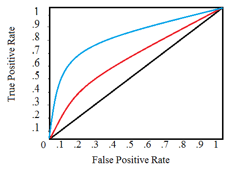
, , . 0 1 . , , . , , , , , , ( ).
(AUC) . ROC ( ). 0 1, . , , ROC AUC = 0,5.
ROC AUC, 0 1, 0 1. , , , ( , ) — . , , 99,9999%, , , . , ( ), , ROC AUC F1, . ROC AUC , ROC AUC .
, , . , , . .
: numpy pandas , sklearn preprocessing , matplotlib ¨C11C¨C12C¨C13C . .
import os
import numpy as np
import pandas as pd
pd.set_option('display.max_columns', None)
from sklearn.preprocessing import LabelEncoder
import matplotlib.pyplot as plt
import seaborn as sns
#
import warnings
warnings.filterwarnings('ignore')
, , . 9 : ( ), ( ), 6 , .
#
print(os.listdir("../input/"))
‘POSCASHbalance.csv’, ‘bureaubalance.csv’, ‘applicationtrain.csv’, ‘previousapplication.csv’, ‘installmentspayments.csv’, ‘creditcardbalance.csv’, ‘samplesubmission.csv’, ‘applicationtest.csv’, ‘bureau.csv’]
#
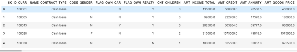
app_train = pd.read_csv('../input/application_train.csv')
print('Training data shape: ', app_train.shape)
app_train.head()
Training data shape: (307511, 122)

307511 , 120 , , .
#
app_test = pd.read_csv('../input/application_test.csv')
print('Testing data shape: ', app_test.shape)
app_test.head()
Testing data shape: (48744, 121)
, TARGET.
(EXPLORATORY DATA ANALYSIS – EDA)
(EDA) — , , , , . EDA — , . , , . , , , , .
— , : 0, , 1, . , .
app_train['TARGET'].value_counts()

app_train['TARGET'].astype(int).plot.hist();
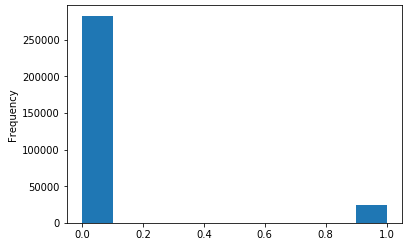
.
#
def missing_values_table(df):
#
mis_val = df.isnull().sum()
#
mis_val_percent = 100 * df.isnull().sum() / len(df)
#
mis_val_table = pd.concat([mis_val, mis_val_percent], axis=1)
#
mis_val_table_ren_columns = mis_val_table.rename(
columns = {0 : 'Missing Values', 1 : '% of Total Values'})
#
mis_val_table_ren_columns = mis_val_table_ren_columns[
mis_val_table_ren_columns.iloc[:,1] != 0].sort_values(
'% of Total Values', ascending=False).round(1)
#
print("Your selected dataframe has " + str(df.shape[1]) + " columns.\n"
"There are " + str(mis_val_table_ren_columns.shape[0]) +
" columns that have missing values.")
return mis_val_table_ren_columns
#
missing_values = missing_values_table(app_train)
missing_values.head(10)
Your selected dataframe has 122 columns.
There are 67 columns that have missing values.

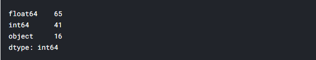
. int64 float64 — ( ). object .
#
app_train.dtypes.value_counts()
object().
#
app_train.select_dtypes('object').apply(pd.Series.nunique, axis = 0)

, . .
, . , ( , LightGBM). , () , . :
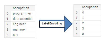
(Label encoding): . . :
(One-hot encoding): . 1 0 .

, . , , - . 4, — 1, , . . , , (, = 4 = 1) , , . (, / ), , .
, , . – Kaggle-master Will Koehrsen, , , . . , ( ) - . , PCA , ( , ).
Label Encoding 2 One-Hot Encoding 2 . , , , , . - .
Label Encoding One-Hot Encoding
: (dtype == object) , – .
LabelEncoder Scikit-Learn, – pandas get_dummies(df).
# label encoder
le = LabelEncoder()
le_count = 0
#
for col in app_train:
if app_train[col].dtype == 'object':
# 2
if len(list(app_train[col].unique())) <= 2:
# LabelEncoder
le.fit(app_train[col])
#
app_train[col] = le.transform(app_train[col])
app_test[col] = le.transform(app_test[col])
# , LabelEncoder
le_count += 1
print('%d columns were label encoded.' % le_count)
3 columns were label encoded.
# one-hot encoding
app_train = pd.get_dummies(app_train)
app_test = pd.get_dummies(app_test)
print('Training Features shape: ', app_train.shape)
print('Testing Features shape: ', app_test.shape)
raining Features shape: (307511, 243)
Testing Features shape: (48744, 239).
(). , , . . ( , ). , axis = 1, , !
train_labels = app_train['TARGET']
# , ,
app_train, app_test = app_train.align(app_test, join = 'inner', axis = 1)
#
app_train['TARGET'] = train_labels
print('Training Features shape: ', app_train.shape)
print('Testing Features shape: ', app_test.shape)
Training Features shape: (307511, 240)
Testing Features shape: (48744, 239)
, . «» . - , , ( , ), .
, EDA, — . - , , . describe. DAYS_BIRTH , . , -1 :
(app_train['DAYS_BIRTH'] / -365).describe()

— . .
app_train['DAYS_EMPLOYED'].describe()
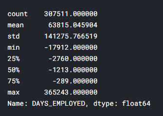
– ( , ) — 1000 !
app_train['DAYS_EMPLOYED'].plot.hist(title = 'Days Employment Histogram');
plt.xlabel('Days Employment');
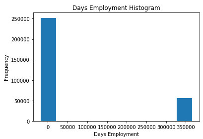
, .
anom = app_train[app_train['DAYS_EMPLOYED'] == 365243]
non_anom = app_train[app_train['DAYS_EMPLOYED'] != 365243]
print('The non-anomalies default on %0.2f%% of loans' % (100 * non_anom['TARGET'].mean()))
print('The anomalies default on %0.2f%% of loans' % (100 * anom['TARGET'].mean()))
print('There are %d anomalous days of employment' % len(anom))
The non-anomalies default on 8.66% of loans
The anomalies default on 5.40% of loans
There are 55374 anomalous days of employment
– , .
. — , . , , , - . , , , . (np.nan), , , .
# ,
app_train['DAYS_EMPLOYED_ANOM'] = app_train["DAYS_EMPLOYED"] == 365243
# nan
app_train['DAYS_EMPLOYED'].replace({365243: np.nan}, inplace = True)
app_train['DAYS_EMPLOYED'].plot.hist(title = 'Days Employment Histogram');
plt.xlabel('Days Employment');

, . , , ( nans , , ). DAYS , , .
: , , . np.nan .
app_test['DAYS_EMPLOYED_ANOM'] = app_test["DAYS_EMPLOYED"] == 365243
app_test["DAYS_EMPLOYED"].replace({365243: np.nan}, inplace = True)
print('There are %d anomalies in the test data out of %d entries' % (app_test["DAYS_EMPLOYED_ANOM"].sum(), len(app_test)))
There are 9274 anomalies in the test data out of 48744 entries
, , EDA. — . , .corr.
.00–0.19 « »
.20-.39 «»
.40–0.59 «»
0,60–0,79 «»
0,80–1,0 « »
#
correlations = app_train.corr()['TARGET'].sort_values()
#
print('Most Positive Correlations:\n', correlations.tail(15))
print('\nMost Negative Correlations:\n', correlations.head(15))
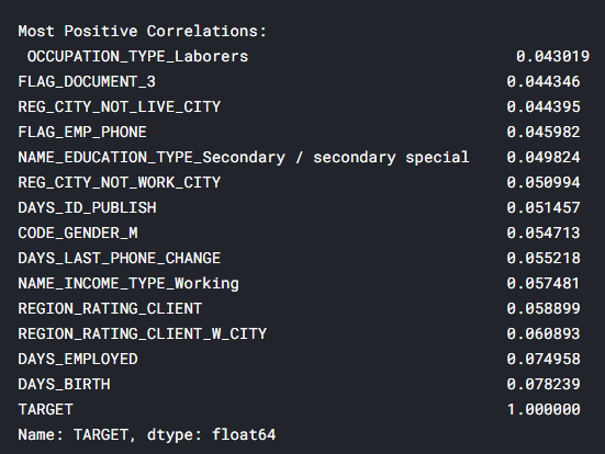
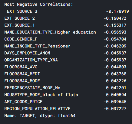
: DAYSBIRTH — ( TARGET, 1). , DAYSBIRTH — . , , , , , (.. == 0). , , .
app_train['DAYS_BIRTH'] = abs(app_train['DAYS_BIRTH'])
app_train['DAYS_BIRTH'].corr(app_train['TARGET'])
-0.07823930830982694
, , , , .
. -, . , x .
plt.style.use('fivethirtyeight')
#
plt.hist(app_train['DAYS_BIRTH'] / 365, edgecolor = 'k', bins = 25)
plt.title('Age of Client'); plt.xlabel('Age (years)'); plt.ylabel('Count');
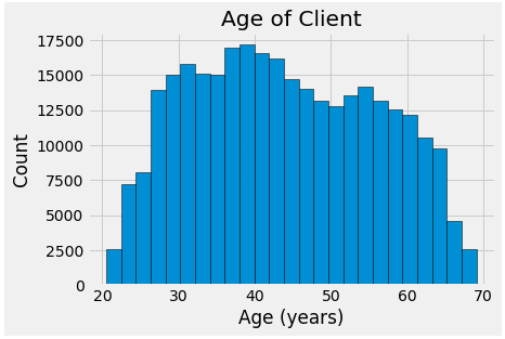
, , , . , (KDE), . ( , , , ). seaborn kdeplot.
plt.figure(figsize = (10, 8))
sns.kdeplot(app_train.loc[app_train['TARGET'] == 0, 'DAYS_BIRTH'] / 365, label = 'target == 0')
sns.kdeplot(app_train.loc[app_train['TARGET'] == 1, 'DAYS_BIRTH'] / 365, label = 'target == 1')
plt.xlabel('Age (years)'); plt.ylabel('Density'); plt.title('Distribution of Ages');
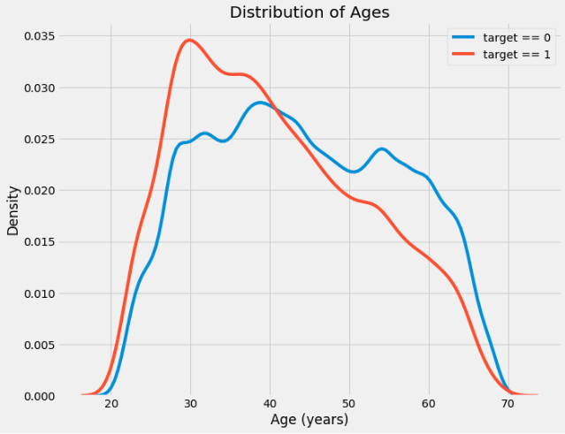
target == 1 . ( -0,07), , , , . : .
, 5 . , .
age_data = app_train[['TARGET', 'DAYS_BIRTH']]
age_data['YEARS_BIRTH'] = age_data['DAYS_BIRTH'] / 365
age_data['YEARS_BINNED'] = pd.cut(age_data['YEARS_BIRTH'], bins = np.linspace(20, 70, num = 11))
age_data.head(10)

#
age_groups = age_data.groupby('YEARS_BINNED').mean()
age_groups

plt.figure(figsize = (8, 8))
plt.bar(age_groups.index.astype(str), 100 * age_groups['TARGET'])
plt.xticks(rotation = 75); plt.xlabel('Age Group (years)'); plt.ylabel('Failure to Repay (%)')
plt.title('Failure to Repay by Age Group');

: . 10% 5% .
: , , . , , , .
: EXTSOURCE1, EXTSOURCE2 EXTSOURCE3. , « ». , , , , , .
.
-, EXT_SOURCE .
ext_data = app_train[['TARGET', 'EXT_SOURCE_1', 'EXT_SOURCE_2', 'EXT_SOURCE_3', 'DAYS_BIRTH']]
ext_data_corrs = ext_data.corr()
ext_data_corrs

plt.figure(figsize = (8, 6))
#
sns.heatmap(ext_data_corrs, cmap = plt.cm.RdYlBu_r, vmin = -0.25, annot = True, vmax = 0.6)
plt.title('Correlation Heatmap');
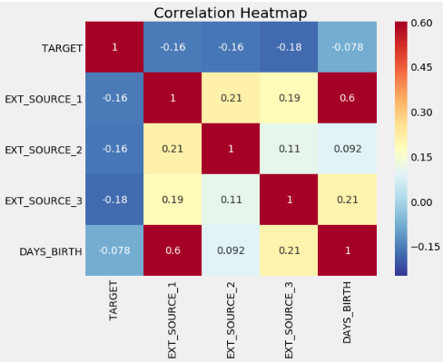
EXT_SOURCE , , EXT_SOURCE . , DAYS_BIRTH EXT_SOURCE_1, , , , .
, . .
plt.figure(figsize = (10, 12))
for i, source in enumerate(['EXT_SOURCE_1', 'EXT_SOURCE_2', 'EXT_SOURCE_3']):
plt.subplot(3, 1, i + 1)
sns.kdeplot(app_train.loc[app_train['TARGET'] == 0, source], label = 'target == 0')
sns.kdeplot(app_train.loc[app_train['TARGET'] == 1, source], label = 'target == 1')
plt.title('Distribution of %s by Target Value' % source)
plt.xlabel('%s' % source); plt.ylabel('Density');
plt.tight_layout(h_pad = 2.5)
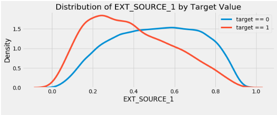
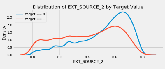
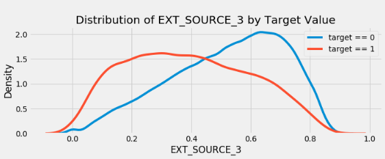
EXT_SOURCE_3 . , . ( ), , , .
EXTSOURCE DAYSBIRTH. – , , . seaborn PairGrid, , 2D .
plot_data = ext_data.drop(columns = ['DAYS_BIRTH']).copy()
plot_data['YEARS_BIRTH'] = age_data['YEARS_BIRTH']
plot_data = plot_data.dropna().loc[:100000, :]
#
def corr_func(x, y, **kwargs):
r = np.corrcoef(x, y)[0][1]
ax = plt.gca()
ax.annotate("r = {:.2f}".format(r),
xy=(.2, .8), xycoords=ax.transAxes,
size = 20)
#
grid = sns.PairGrid(data = plot_data, size = 3, diag_sharey=False,
hue = 'TARGET',
vars = [x for x in list(plot_data.columns) if x != 'TARGET'])
grid.map_upper(plt.scatter, alpha = 0.2)
grid.map_diag(sns.kdeplot)
grid.map_lower(sns.kdeplot, cmap = plt.cm.OrRd_r);
plt.suptitle('Ext Source and Age Features Pairs Plot', size = 32, y = 1.05);
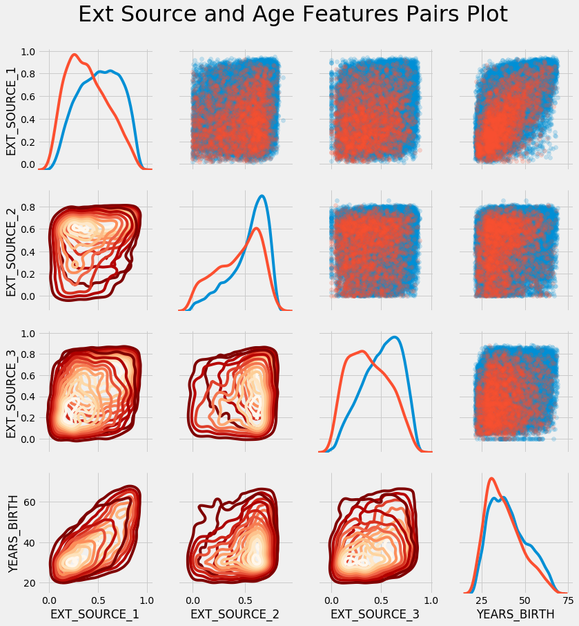
In dieser Grafik zeigt Rot Kredite an, die nicht zurückgezahlt wurden, und Blau zeigt Kredite an, die zurückgezahlt wurden. Wir können verschiedene Beziehungen in den Daten sehen. Es gibt tatsächlich eine moderat positive lineare Beziehung zwischen EXT_SOURCE_1 und YEARS_BIRTH, was darauf hinweist, dass dieses Merkmal altersspezifisch sein kann.
Damit ist der erste Artikel abgeschlossen. Im nächsten Teil werde ich über die Entwicklung zusätzlicher Funktionen basierend auf den verfügbaren Daten sprechen und auch zeigen, wie ein einfaches Modell für maschinelles Lernen erstellt wird.
Bei der Erstellung des Artikels wurden Materialien aus Open Source verwendet: source_1 , source_2 .