In einer guten Stadt in der Nähe von Moskau gibt es einen schlechten Bahnübergang. Während der Hauptverkehrszeit steigt es nicht nur, sondern auch benachbarte Kreuzungen und Straßen. Beim erneuten Fahren fragte ich mich: Was ist seine Kapazität und kann etwas geändert werden?

Zur Beantwortung werden wir uns ein wenig mit den Vorschriften und der Theorie der Verkehrsströme befassen, die GPS- und Beschleunigungsmesserdaten mit Python analysieren und die theoretischen Berechnungen mit den experimentellen Daten vergleichen.
Inhalt
1.
, 10 /. .
Jupyter Notebook GitHub'.

:
import pandas as pd
import numpy as np
import glob

#!pip install utm
import utm

from sklearn.decomposition import PCA
from scipy import interpolate

import matplotlib.pyplot as plt
import seaborn as sns
sns.set(rc={'figure.figsize':(12, 8)})
import plotly.express as px

#  Mapbox    Plotly
mapbox_token = open('mapbox_token', 'r').read()
2.
.
— 1 .
— .
— , .
— , - .
:
.
« » . , 2005 . , .

218.2.020-2012 " ".
, :
— , , , .
, :
, , .
2 :
- ;
- .
:
- :
,
,
– () , – , – , , — . ( ): .
- :
,
— ( ), — () ( ). 218.2.020-2012 —
#
diagram1 = pd.read_csv('  .csv', sep=';', header=None, names=['P', 'V'], decimal=',')
diagram1_func = interpolate.interp1d(diagram1['P'], diagram1['V'], kind='cubic')
diagram1_xnew = np.arange(diagram1['P'].min(), diagram1['P'].max())

#
diagram2 = pd.read_csv(' .csv', sep=';', header=None, names=['P', 'Q'], decimal=',')
diagram2_func = interpolate.interp1d(diagram2['P'], diagram2['Q'], kind='cubic')
diagram2_xnew = np.arange(diagram2['P'].min(), diagram2['P'].max())
def density_Tanaka(V):
#
V = V * 1000 / 60 / 60 # / /
L = 5.7 #
c1 = 0.504 #
c2 = 0.0285 #**2/
return 1000 / (L + c1 * V + c2 * V**2) # ./
def density_Grindshilds(V):
#
pmax = 85 # ./
vmax = 60 # /
return pmax * (1 - V / vmax) # ./#
V = np.arange(1, 80) # /
V1 = np.arange(1, 61) # /
fig, (ax1, ax2) = plt.subplots(1, 2, figsize=(16, 8))
ax1.plot(density_Tanaka(V), V, label=" ")
ax1.plot(density_Grindshilds(V1), V1, label=" ")
ax1.plot(diagram1_xnew, diagram1_func(diagram1_xnew), label=". ")
ax1.set_xlabel(r' $\rho$, /')
ax1.set_ylabel(r' $V$, /')
ax1.legend()
ax2.plot(density_Tanaka(V), density_Tanaka(V) * V, label=" ")
ax2.plot(density_Grindshilds(V1), density_Grindshilds(V1) * V1, label=" ")
ax2.plot(diagram2_xnew, diagram2_func(diagram2_xnew), label=". ")
ax2.set_xlabel(r' $\rho$, /')
ax2.set_ylabel(r' $Q$, /')
ax2.legend()
plt.show()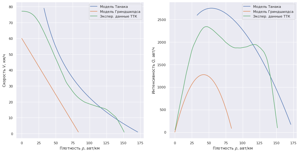
. .
3.
3.1
, . Enter, :
%%writefile "key-logger.py"
import pandas as pd
import time
import datetime

class _GetchUnix:
    # from https://code.activestate.com/recipes/134892/
    def __init__(self):
        import tty, sys

    def __call__(self):
        import sys, tty, termios
        fd = sys.stdin.fileno()
        old_settings = termios.tcgetattr(fd)
        try:
            tty.setraw(sys.stdin.fileno())
            ch = sys.stdin.read(1)
        finally:
            termios.tcsetattr(fd, termios.TCSADRAIN, old_settings)
        return ch

def logging():
    path = 'logs/keylog/'
    filename = f"{time.strftime('%Y-%m-%d %H-%M-%S')}.csv"
    path_to_file = path + filename
    db = []
    getch = _GetchUnix()
    print('...')
    while True:
        key = getch()
        if key == 'c':
            break
        else:
            db.append((datetime.datetime.now(), key))
    df = pd.DataFrame(db, columns=['time', 'click'])
    print(df)
    df.to_csv(path_to_file, index=False)
    print(f"\nSaved to {filename}")

if __name__ == "__main__":
    logging()
20 . 2 , . . 100%:
files = glob.glob('logs/keylog/*.csv')
keylogger_data = []
print(f'  - {len(files)} .')
for filename in files:
    df = pd.read_csv(filename, parse_dates=['time'])
    keylogger_data.append(df)
keylogger_data = pd.concat(keylogger_data, ignore_index=True)
keylogger_data.head()| time | click | |
|---|---|---|
| 0 | 2020-09-29 16:24:02.691189 | d |
| 1 | 2020-09-29 16:24:05.186670 | a |
| 2 | 2020-09-29 16:24:07.157702 | d |
| 3 | 2020-09-29 16:24:11.506961 | a |
| 4 | 2020-09-29 16:24:14.206266 | a |
"a" — , 'd' — .
:
keylogger_data['time'] = keylogger_data['time'].astype('datetime64[m]')
keylogger_per_min = keylogger_data.groupby(['click', 'time'], as_index=False).size().reset_index().rename(columns={0:'size'})
keylogger_per_min.head()| index | click | time | size | |
|---|---|---|---|---|
| 0 | 0 | a | 2020-09-29 16:24:00 | 12 |
| 1 | 1 | a | 2020-09-29 16:25:00 | 13 |
| 2 | 2 | a | 2020-09-29 16:26:00 | 9 |
| 3 | 3 | a | 2020-09-29 16:27:00 | 18 |
| 4 | 4 | a | 2020-09-29 16:28:00 | 14 |
sns.catplot(x='click', y='size', kind="box", data=keylogger_per_min);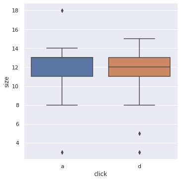
print(f"  : {keylogger_per_min['size'].mean():.1f} ./ \
 {keylogger_per_min['size'].mean() * 60:.1f} ./")
: 11.7 ./ 700.0 ./
.
— 700 ./ 10 / ( 50 / ) — .
plt.plot(V1, density_Grindshilds(V1)*V1, label=" ")
plt.xlabel(r' $V$, /')
plt.ylabel(r' $Q$, /')
plt.show()
3.2
Android GPSLogger csv . ( ) GPS — Physics Toolbox Suite.
50 . — .
, — .
GPSLogger
GPSLogger , :
- time — ;
- lat lon — , ;
- speed — , ;
- direction — , .
files = glob.glob('logs/gps/*.csv')
gpslogger_data = []
print(f'    GPS - {len(files)} .')
for filename in files:
    df = pd.read_csv(filename, parse_dates=['time'], index_col='time')
    if df.iloc[10, 1] < df.iloc[-1, 1]:
        df['direction'] = 0 #
    else:
        df['direction'] = 1 #
    gpslogger_data.append(df)
gpslogger_data = pd.concat(gpslogger_data)
gpslogger_data.head()

gps_1 = gpslogger_data[['lat', 'lon', 'speed', 'direction']]
GPS — 37 .
Physics Toolbox Suite:
files = glob.glob('logs/gps_accel/*.csv')
print(f'     - {len(files)} .')
pts_data = []

for filename in files:
    df = pd.read_csv(filename, sep=';',decimal=',')
    df['time'] = filename[-22:-12] + '-' + df['time']
    if df.iloc[10, 5] < df.iloc[-1, 5]:
        df['direction'] = 0 #
    else:
        df['direction'] = 1 #
    pts_data.append(df)
pts_data = pd.concat(pts_data)
pts_data.head()
— 14 .
| time | ax | ay | az | Latitude | Longitude | Speed (m/s) | Unnamed: 7 | direction | |
|---|---|---|---|---|---|---|---|---|---|
| 0 | 2020-09-04-14:11:18:029 | 0.0 | 0.0 | 0.0 | 0.000000 | 0.00000 | 0.0 | NaN | 1 |
| 1 | 2020-09-04-14:11:18:030 | 0.0 | 0.0 | 0.0 | 56.372343 | 37.53044 | 0.0 | NaN | 1 |
| 2 | 2020-09-04-14:11:18:030 | 0.0 | 0.0 | 0.0 | 56.372343 | 37.53044 | 0.0 | NaN | 1 |
| 3 | 2020-09-04-14:11:18:094 | 0.0 | 0.0 | 0.0 | 56.372343 | 37.53044 | 0.0 | NaN | 1 |
| 4 | 2020-09-04-14:11:18:094 | 0.0 | 0.0 | 0.0 | 56.372343 | 37.53044 | 0.0 | NaN | 1 |
, — :
pts_data = pts_data.query('Latitude != 0.')Physics Toolbox Suite 400 , GPS 1 , :
pts_data['time'] = pd.to_datetime(pts_data['time'], format='%Y-%m-%d-%H:%M:%S:%f')
pts_data = pts_data.rename(columns={'Latitude':'lat', 'Longitude':'lon', 'Speed (m/s)':'speed'})
:
accel_data = pts_data[['time', 'lat', 'lon', 'ax', 'ay', 'az', 'direction']].copy()
accel_data = accel_data.set_index('time')
accel_data['direction'] = accel_data['direction'].map({1.: ' ', 0.: ' '})
accel_data.head()| lat | lon | ax | ay | az | direction | |
|---|---|---|---|---|---|---|
| time | ||||||
| 2020-09-04 14:11:18.030 | 56.372343 | 37.53044 | 0.0 | 0.0 | 0.0 | |
| 2020-09-04 14:11:18.030 | 56.372343 | 37.53044 | 0.0 | 0.0 | 0.0 | |
| 2020-09-04 14:11:18.094 | 56.372343 | 37.53044 | 0.0 | 0.0 | 0.0 | |
| 2020-09-04 14:11:18.094 | 56.372343 | 37.53044 | 0.0 | 0.0 | 0.0 | |
| 2020-09-04 14:11:18.095 | 56.372343 | 37.53044 | 0.0 | 0.0 | -0.0 |
GPS:
gps_2 = pts_data[['time', 'lat', 'lon', 'speed', 'direction']].copy()
gps_2 = gps_2.set_index('time')
gps_2 = gps_2.resample('S').mean()
gps_2 = gps_2.dropna(how='all')
gps_2.head()| lat | lon | speed | direction | |
|---|---|---|---|---|
| time | ||||
| 2020-08-10 00:45:02 | 56.338342 | 37.522946 | 0.0 | 1.0 |
| 2020-08-10 00:45:03 | 56.338342 | 37.522946 | 0.0 | 1.0 |
| 2020-08-10 00:45:04 | 56.338342 | 37.522946 | 0.0 | 1.0 |
| 2020-08-10 00:45:05 | 56.338342 | 37.522946 | 0.0 | 1.0 |
| 2020-08-10 00:45:06 | 56.338342 | 37.522946 | 0.0 | 1.0 |
GPS :
gps_data = gps_1.append(gps_2, ignore_index=True)
gps_data['direction'] = gps_data['direction'].map({1.: ' ', 0.: ' '})
gps_data.head()| lat | lon | speed | direction | |
|---|---|---|---|---|
| 0 | 56.167241 | 37.504026 | 19.82 | |
| 1 | 56.167051 | 37.503804 | 19.36 | |
| 2 | 56.166884 | 37.503667 | 19.62 | |
| 3 | 56.166718 | 37.503554 | 19.35 | |
| 4 | 56.166570 | 37.503427 | 19.12 |
3.2.1
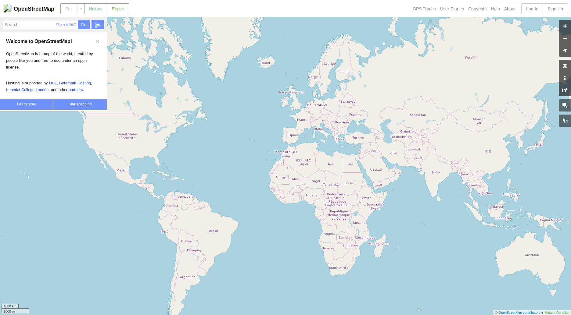
Plotly:
fig = px.scatter_mapbox(gps_data, lat="lat", lon="lon", color='direction', zoom=17, height=600)
fig.update_layout(mapbox_accesstoken=mapbox_token, mapbox_style='streets')
fig.show()
3.2.2
:
- GPS, WGS 84 .
- .
Web Mercator, — , , .
, . — , — (UTM).
Web-Mercator
UTM
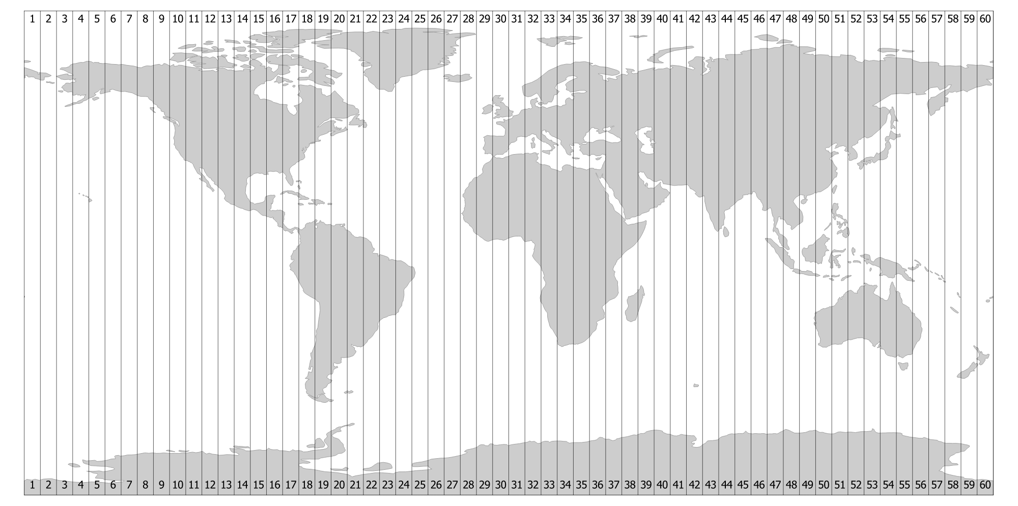
UTM Python https://github.com/Turbo87/utm, .
gps_data['xs'] = gps_data[['lat', 'lon']].apply(lambda x: utm.from_latlon(x[0], x[1])[0], axis=1)
gps_data['ys'] = gps_data[['lat', 'lon']].apply(lambda x: utm.from_latlon(x[0], x[1])[1], axis=1)
gps_data['speed_kmh'] = gps_data.speed / 1000 * 60 * 60
50 :
#
lat0 = 56.35205
lon0 = 37.51792
xc, yc, _, _ = utm.from_latlon(lat0, lon0)

r = 50
gps_data = gps_data.query(f'{xc - r} < xs & xs < {xc + r}')\
                   .query(f'{yc - r} < ys & ys < {yc + r}')
fig = px.scatter_mapbox(gps_data, lat="lat", lon="lon", color='direction', zoom=17, height=600)
fig.update_layout(mapbox_accesstoken=mapbox_token, mapbox_style='streets')
fig.show()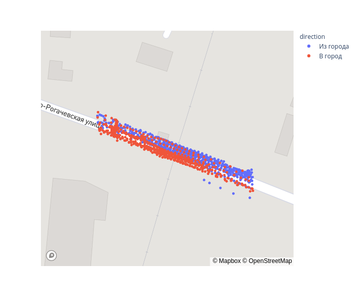
. 2d 1d, (PCA).
2 — scikit-learn. Sklearn:
pca = PCA(n_components=1).fit(gps_data[['xs', 'ys']])
gps_data['xs_transform'] = pca.transform(gps_data[['xs', 'ys']])sns.relplot(x='xs_transform', y='speed_kmh', data=gps_data, aspect=2.5, hue='direction');
. — [-5, 25]. .
accel_data['xs'] = accel_data[['lat', 'lon']].apply(lambda x: utm.from_latlon(x[0], x[1])[0], axis=1)
accel_data['ys'] = accel_data[['lat', 'lon']].apply(lambda x: utm.from_latlon(x[0], x[1])[1], axis=1)
accel_data = accel_data.query(f'{xc - r} < xs & xs < {xc + r}')\
                       .query(f'{yc - r} < ys & ys < {yc + r}')
accel_data['xs_transform'] = pca.transform(accel_data[['xs', 'ys']])
Android :

( Y). :
sns.relplot(x='xs_transform', y='ax', data=accel_data, aspect=2.5, hue='direction');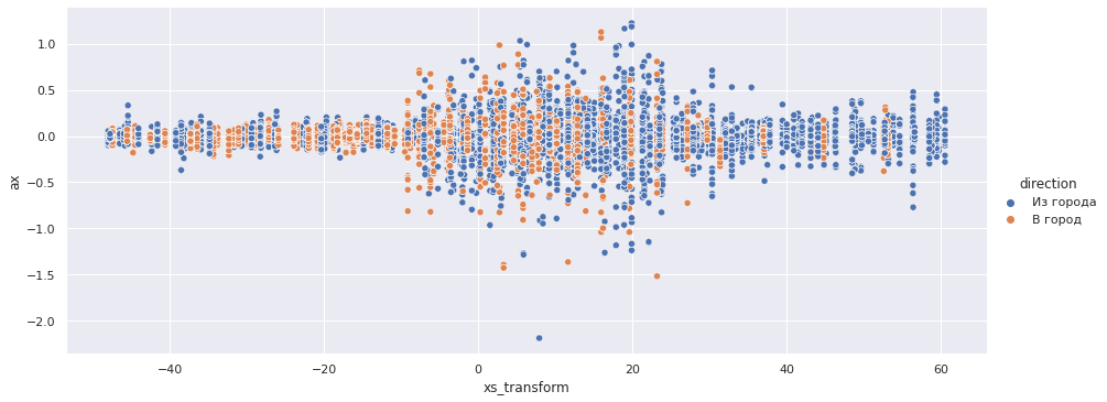
sns.relplot(x='xs_transform', y='ay', data=accel_data, aspect=2.5, hue='direction');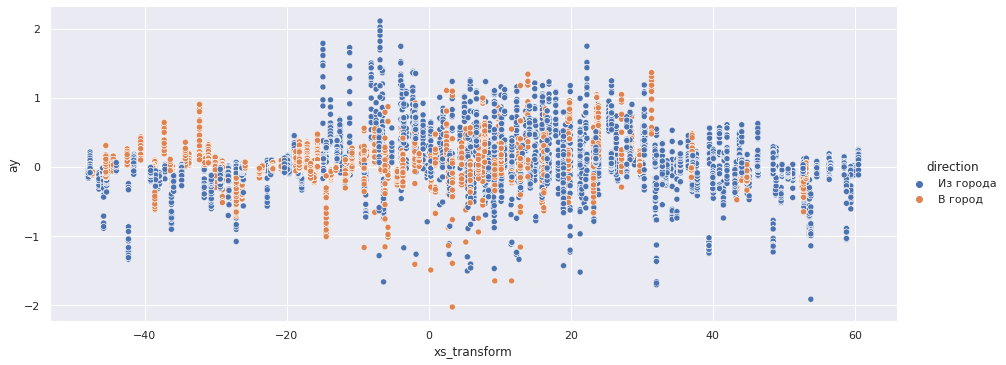
sns.relplot(x='xs_transform', y='az', data=accel_data, aspect=2.5, hue='direction');
Z:
sns.relplot(x='xs_transform', y='az', data=accel_data.query('-20 < xs_transform < 40'), aspect=2.5, hue='direction');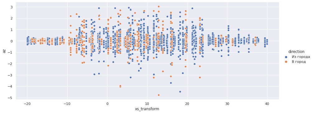
X Z — [-10, 25] 7.5.
cross = gps_data.query('-10 < xs_transform < 25')fig = px.scatter_mapbox(cross, lat="lat", lon="lon", color='direction', zoom=19, height=600)
fig.update_layout(mapbox_accesstoken=mapbox_token, mapbox_style='streets')
fig.show()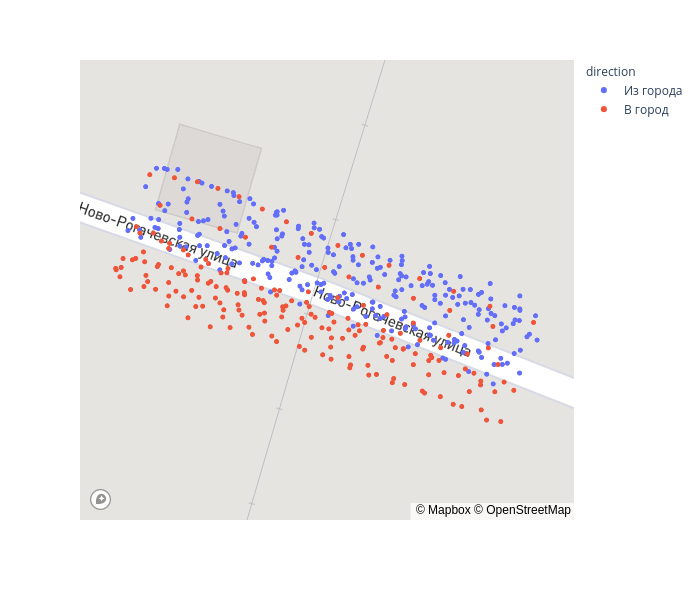
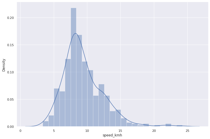
:
mean_v = cross.speed_kmh.mean()
print(f"    - {mean_v:.2} /")
sns.distplot(cross.speed_kmh);
— 9.4 /
:
base = 1
gps_data['xs_transform_round'] = gps_data['xs_transform'].apply(lambda x: base * round(x / base))
accel_data['xs_transform_round'] = accel_data['xs_transform'].apply(lambda x: base * round(x / base))sns.relplot(x='xs_transform_round', y='speed_kmh', data=gps_data, kind="line", aspect=2.5);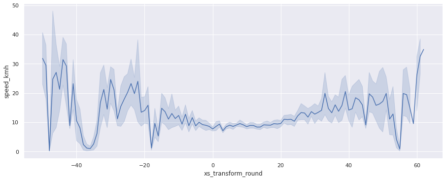
sns.relplot(x='xs_transform_round', y='az', data=accel_data, kind="line", aspect=2.5);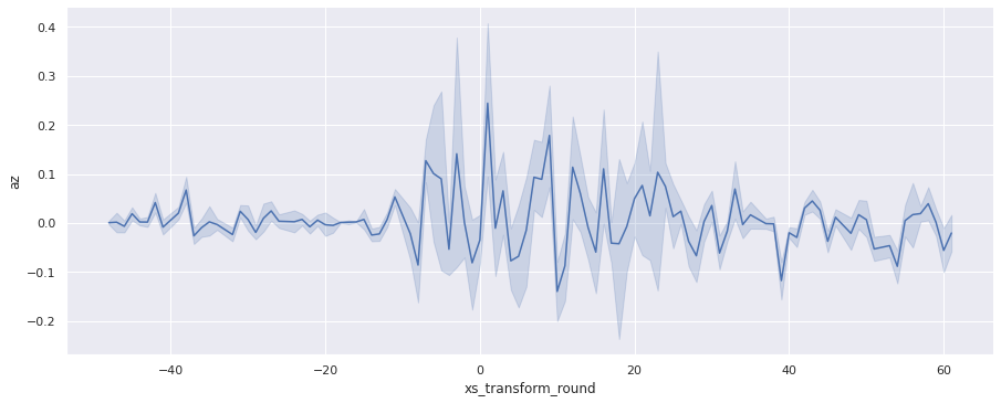
3.3
:
gps_data['flow_Tanaka'] = density_Tanaka(gps_data.speed_kmh) * gps_data.speed_kmh
gps_data['flow_Grindshilds'] = density_Grindshilds(gps_data.speed_kmh) * gps_data.speed_kmhsns.relplot(x='xs_transform_round', y='flow_Grindshilds', data=gps_data, aspect=2.5, kind='line', hue='direction');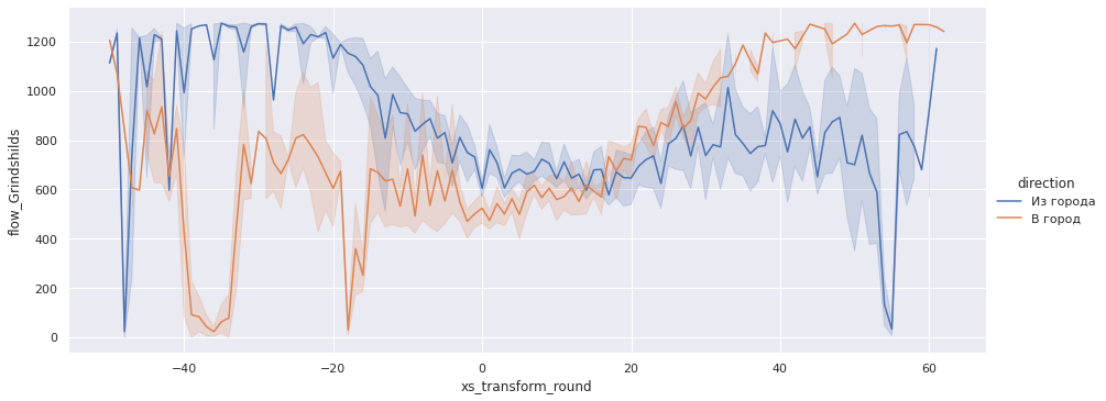
cross = gps_data.query('-10 < xs_transform < 25')mean_flow_Tanaka = cross.flow_Tanaka.mean()
print(f" - {mean_flow_Tanaka:.1f} / \
{mean_flow_Tanaka / 60:.1f} /")— 1275.5 / 21.3 /
mean_flow_Grindshilds = cross.flow_Grindshilds.mean()
print(f"      - {mean_flow_Grindshilds:.1f} / \
 {mean_flow_Grindshilds / 60:.1f} /")
— 660.0 / 11.0 /
, 700 ./.
plt.plot(V1, density_Grindshilds(V1)*V1, label=" ")
plt.xlabel(r' $V$, /')
plt.ylabel(r' $Q$, /')
plt.show()
, - 30 / — .
, :
4.
Basierend auf unserer Analyse kann argumentiert werden, dass sich der Bahnübergang in einem unbefriedigenden Zustand befindet und die Durchflussrate etwa 10 km / h beträgt, was bei voller Beladung der Straße zu Verkehrsproblemen und Staus führt.
Der Durchsatz der Kreuzung kann erheblich erhöht werden, indem die Kreuzung in einen zufriedenstellenden Zustand gebracht wird.