Black [O] lebt Materie: Rasse, Verbrechen und Feuer, um in den Vereinigten Staaten zu töten. Teil 3

Wir setzen unsere Forschungen zur Situation in den Vereinigten Staaten mit der Erschießung von Polizisten und der Kriminalitätsrate unter Vertretern der weißen und schwarzen (afroamerikanischen) Rassen fort. Ich möchte Sie daran erinnern, dass ich im ersten Teil über die Prämissen der Studie, ihre Ziele und akzeptierten Vorbehalte / Annahmen gesprochen habe. und der zweite Teil war eine Demonstration der Analyse der Beziehung zwischen Rasse, Verbrechen und Tod durch Strafverfolgungsbehörden.

Ich möchte Sie auch an die Zwischenergebnisse erinnern, die auf der Grundlage statistischer Beobachtungen (für den Zeitraum von 2000 bis 2018) gezogen wurden:

• In quantitativen (absoluten) Begriffen gibt es mehr weiße Polizeiopfer als Schwarze.

• Im Durchschnitt tötet die Polizei 5,9 pro Million Schwarze und 2,3 pro Million Weiße (2,6-mal mehr Schwarze).

• Die jährliche Streuung (Abweichung) bei den Todesfällen von Schwarzen durch die Polizei ist fast doppelt so hoch wie bei den Daten für weiße Opfer.

• Die polizeilichen Opfer unter Weißen nehmen monoton zu (im Durchschnitt um 0,1 - 0,2 pro Jahr), während die Opfer unter Schwarzen nach einem Höhepunkt in den Jahren 2011 - 2013 auf das Niveau von 2009 zurückgekehrt sind.

• Weiße begehen in absoluten Zahlen doppelt so viele Verbrechen wie Schwarze, aber relativ gesehen dreimal weniger (pro Million Mitglieder ihrer Rasse).

• Das weiße Verbrechen hat während des gesamten Zeitraums relativ eintönig zugenommen (es hat sich in 18 Jahren verdoppelt). Das schwarze Verbrechen nimmt ebenfalls zu, jedoch sprunghaft. Während des gesamten Zeitraums verdoppelte sich auch die Kriminalität unter Schwarzen (ähnlich wie bei Weißen).

• Der Tod durch die Polizei ist mit Kriminalität verbunden (die Anzahl der begangenen Verbrechen). Darüber hinaus ist diese Korrelation zwischen den Rassen heterogen: Für Weiße ist sie nahezu ideal, für Schwarze ist sie weit davon entfernt.

• Todesfälle bei Treffen mit der Polizei nehmen "als Reaktion" auf die Zunahme der Kriminalität mit einer Verzögerung von mehreren Jahren zu (insbesondere in den Daten unter Schwarzen).

• Weiße Kriminelle werden etwas häufiger von der Polizei getötet als schwarze.

, , , , , .

, , , , " " (All Offenses) "". , , " " , , , ( ) , . , (, , )... , !

" "

, , ,

df_crimes1 = df_crimes1.loc[df_crimes1['Offense'] == 'All Offenses']

:

df_crimes1 = df_crimes1.loc[df_crimes1['Offense'].str.contains('Assault|Murder')]

, , (Assault) (Murder). , , .

. .

:

, , ( ).

:

:

, (0.68 0.88 0.72 ). , , , .. , .

, "" - :

, . - , .

, .

, - ! :)

, :

• (State level UCR Estimated Crime Data Endpoint) - (CSV );

• (State level Arrest Demographic Count By Offense Endpoint) - (CSV ).

, , , : , , . .

51 1991 2018 , :

1. violent crime: (, , ), . ;

2. homicide:

3. rape legacy: ( - 2013 .)

4. rape revised: ( - 2013 .)

5. robbery:

6. aggravated assault:

7. property crime:

8. burglary: /

9. larceny:

10. motor vehicle theft:

11. arson:

(violent crime), .

51 2000 2018 , ( - . ). , 4 (, , ).

:

import pandas as pd, numpy as np

CRIME_STATES_FILE = ROOT_FOLDER + '\\crimes_by_state.csv'
df_crime_states = pd.read_csv(CRIME_STATES_FILE, sep=';', header=0, 
                              usecols=['year', 'state_abbr', 'population', 'violent_crime'])

:

1428 rows × 4 columns

(CSV - ). :

df_crime_states = df_crime_states.merge(df_state_names, on='state_abbr')
df_crime_states.dropna(inplace=True)
df_crime_states.sort_values(by=['year', 'state_abbr'], inplace=True)

, :

df_crime_states['crime_promln'] = df_crime_states['violent_crime'] * 1e6 / df_crime_states['population']

, 2000 2018 , :

df_crime_states_agg = df_crime_states.groupby(['state_name', 'year'])['violent_crime'].sum().unstack(level=1).T
df_crime_states_agg.fillna(0, inplace=True)
df_crime_states_agg = df_crime_states_agg.astype('uint32').loc[2000:2018, :]

19 ( , .. 2000 2018) 51 ( ).

-10 :

df_crime_states_top10 = df_crime_states_agg.describe().T.nlargest(10, 'mean').astype('int32')

:

df_crime_states_top10 = df_crime_states_agg.loc[:, df_crime_states_agg_top10.index]
plt = df_crime_states_top10.plot.box(figsize=(12, 10))
plt.set_ylabel('-   (2000 - 2018)')

"" . - (, ); :)

, (, , ), (, ).

, . -10 2018 :

df_crime_states_2018 = df_crime_states.loc[df_crime_states['year'] == 2018]
plt = df_crime_states_2018.nlargest(10, 'population').sort_values(by='population').plot.barh(x='state_name', y='population', legend=False, figsize=(10,5))
plt.set_xlabel(' (2018)')
plt.set_ylabel('')

, , . :

#      2000 - 2018  (   )
df_corr = df_crime_states[df_crime_states['year']>=2000].groupby(['state_name']).mean()
#     ""  "- "
df_corr = df_corr.loc[:, ['population', 'violent_crime']]
df_corr.corr(method='pearson').at['population', 'violent_crime']

- 0.98. !

-:

plt = df_crime_states_2018.nlargest(10, 'crime_promln').sort_values(by='crime_promln').plot.barh(x='state_name', y='crime_promln', legend=False, figsize=(10,5))
plt.set_xlabel('-    1 . . (2018)')
plt.set_ylabel('')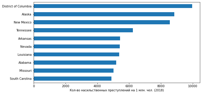

! : (.. ) ( 700+ . 2018 .) (- 2 . .) , , , ...

. folium:

import folium

- 2018 . :

FOLIUM_URL = 'https://raw.githubusercontent.com/python-visualization/folium/master/examples/data'
FOLIUM_US_MAP = f'{FOLIUM_URL}/us-states.json'

m = folium.Map(location=[48, -102], zoom_start=3)

folium.Choropleth(
    geo_data=FOLIUM_US_MAP,
    name='choropleth',
    data=df_crime_states_2018,
    columns=['state_abbr', 'violent_crime'],
    key_on='feature.id',
    fill_color='YlOrRd',
    fill_opacity=0.7,
    line_opacity=0.2,
    legend_name='   2018 .',
    bins=df_crime_states_2018['violent_crime'].quantile(list(np.linspace(0.0, 1.0, 5))).to_list(),
    reset=True
).add_to(m)

folium.LayerControl().add_to(m)

m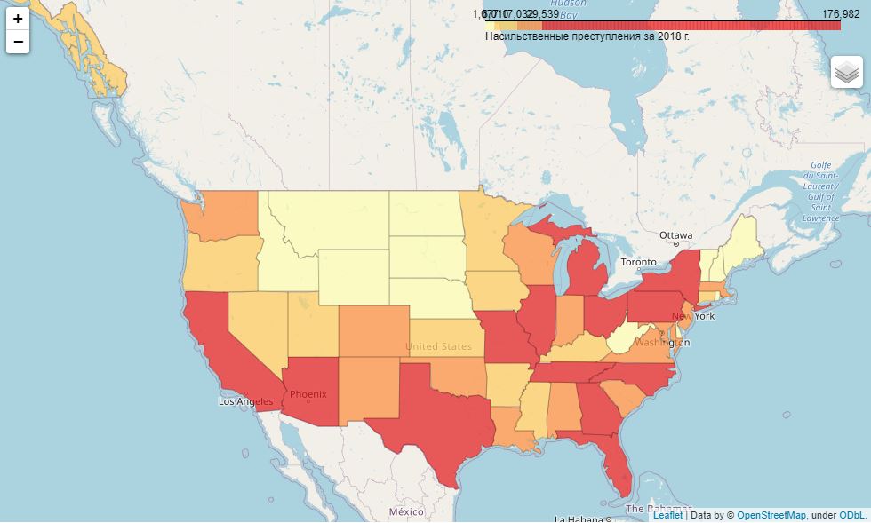

( 1 ):

m = folium.Map(location=[48, -102], zoom_start=3)

folium.Choropleth(
    geo_data=FOLIUM_US_MAP,
    name='choropleth',
    data=df_crime_states_2018,
    columns=['state_abbr', 'crime_promln'],
    key_on='feature.id',
    fill_color='YlOrRd',
    fill_opacity=0.7,
    line_opacity=0.2,
    legend_name='   2018 . ( 1 . )',
    bins=df_crime_states_2018['crime_promln'].quantile(list(np.linspace(0.0, 1.0, 5))).to_list(),
    reset=True
).add_to(m)

folium.LayerControl().add_to(m)

m

, , - .

( )

, .

: (. ) , , 2000 2018 .

df_fenc_agg_states = df_fenc.merge(df_state_names, how='inner', left_on='State', right_on='state_abbr')
df_fenc_agg_states.fillna(0, inplace=True)
df_fenc_agg_states = df_fenc_agg_states.rename(columns={'state_name_x': 'State Name'})
df_fenc_agg_states = df_fenc_agg_states.loc[:, ['Year', 'Race', 'State', 'State Name', 'Cause', 'UOF']]
df_fenc_agg_states = df_fenc_agg_states.groupby(['Year', 'State Name', 'State'])['UOF'].count().unstack(level=0)
df_fenc_agg_states.fillna(0, inplace=True)
df_fenc_agg_states = df_fenc_agg_states.astype('uint16').loc[:, :2018]
df_fenc_agg_states = df_fenc_agg_states.reset_index()

-10 2018 :

df_fenc_agg_states_2018 = df_fenc_agg_states.loc[:, ['State Name', 2018]]
plt = df_fenc_agg_states_2018.nlargest(10, 2018).sort_values(2018).plot.barh(x='State Name', y=2018, legend=False, figsize=(10,5))
plt.set_xlabel('-      2018 .')
plt.set_ylabel('')

" ":

fenc_top10 = df_fenc_agg_states.loc[df_fenc_agg_states['State Name'].isin(df_fenc_agg_states_2018.nlargest(10, 2018)['State Name'])]
fenc_top10 = fenc_top10.T
fenc_top10.columns = fenc_top10.loc['State Name', :]
fenc_top10 = fenc_top10.reset_index().loc[2:, :].set_index('Year')
df_sorted = fenc_top10.mean().sort_values(ascending=False)
fenc_top10 = fenc_top10.loc[:, df_sorted.index]

plt = fenc_top10.plot.box(figsize=(12, 6))
plt.set_ylabel('-     (2000 - 2018)')

, " ": , - . , , , .

, . , .

( ) , 2000 2018 ( ).

#       
df_fenc_crime_states = df_fenc.merge(df_state_names, how='inner', left_on='State', right_on='state_abbr')
#  
df_fenc_crime_states = df_fenc_crime_states.rename(columns={'Year': 'year', 'state_name_x': 'state_name'})
#    2000-2018
df_fenc_crime_states = df_fenc_crime_states[df_fenc_crime_states['year'].between(2000, 2018)]
#       
df_fenc_crime_states = df_fenc_crime_states.groupby(['year', 'state_name'])['UOF'].count().reset_index()
#    
df_fenc_crime_states = df_fenc_crime_states.merge(df_crime_states[df_crime_states['year'].between(2000, 2018)], how='outer', on=['year', 'state_name'])
#   
df_fenc_crime_states.fillna({'UOF': 0}, inplace=True)
#   
df_fenc_crime_states = df_fenc_crime_states.astype({'year': 'uint16', 'UOF': 'uint16', 'population': 'uint32', 'violent_crime': 'uint32'})
# 
df_fenc_crime_states = df_fenc_crime_states.sort_values(by=['year', 'state_name'])

, UOF ( "Use Of Force" - ) ( "", , ) .

:

df_fenc_crime_states_agg = df_fenc_crime_states.groupby(['state_name']).mean().loc[:, ['UOF', 'violent_crime']]

( ):

plt = df_fenc_crime_states_agg['violent_crime'].plot.bar(legend=True, figsize=(15,5))
plt.set_ylabel(' -  ')
plt2 = df_fenc_crime_states_agg['UOF'].plot(secondary_y=True, style='g', legend=True)
plt2.set_ylabel(' -    ', rotation=90)
plt2.set_xlabel('')
plt.set_xlabel('')
plt.set_xticklabels(df_fenc_crime_states_agg.index, rotation='vertical')
plt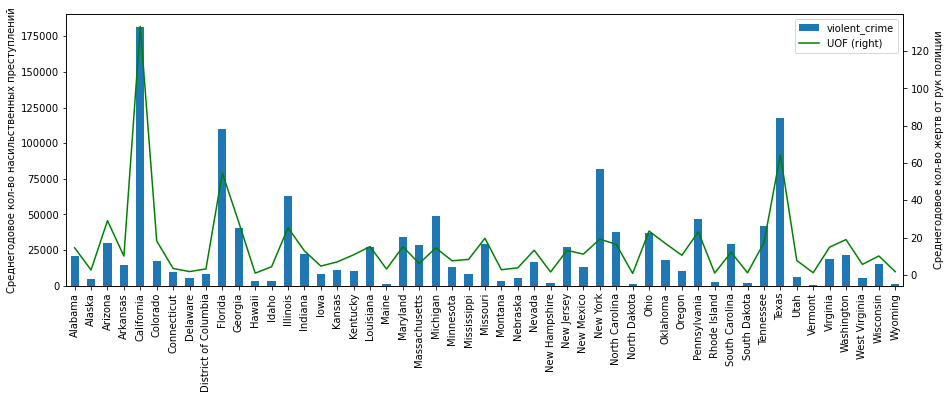

, :

• " ": "" ;

• (, , , -, ) ( ) .

:

plt = df_fenc_crime_states_agg.plot.scatter(x='violent_crime', y='UOF')
plt.set_xlabel(' -  ')
plt.set_ylabel(' -    ')

, . , 75 . , 75 . "" , , . " ":

df_fenc_crime_states_agg[df_fenc_crime_states_agg['violent_crime'] > 75000]

, " ": , , -.

3 :

1. 75 .

2. 75 . ( "")

:

df_fenc_crime_states_agg[df_fenc_crime_states_agg['violent_crime'] <= 75000].corr(method='pearson').at['UOF', 'violent_crime']

0.839. , 0.9 , 47 .

:

df_fenc_crime_states_agg[df_fenc_crime_states_agg['violent_crime'] > 75000].corr(method='pearson').at['UOF', 'violent_crime']

0.999 - !

( ):

df_fenc_crime_states_agg.corr(method='pearson').at['UOF', 'violent_crime']

: 0.935. .

, " " (, , ). , , :

df_fenc_crime_states_agg['uof_by_crime'] = df_fenc_crime_states_agg['UOF'] / df_fenc_crime_states_agg['violent_crime']
plt = df_fenc_crime_states_agg.loc[:, 'uof_by_crime'].sort_values(ascending=False).plot.bar(figsize=(15,5))
plt.set_xlabel('')
plt.set_ylabel(' -    - ')

, , , "" ( ).

:

1. (, !)

2. - : , , -.

2. ( ) , , - (. ).

3. , 0.93 . (.. ), - 0.84.

, , , . , , , . , , , , . . , (, , ), .

CSV :

ARRESTS_FILE = ROOT_FOLDER + '\\arrests_by_state_race.csv'
#      
df_arrests = pd.read_csv(ARRESTS_FILE, sep=';', header=0, usecols=['data_year', 'state', 'white', 'black'])
#    4      
df_arrests = df_arrests.groupby(['data_year', 'state']).sum().reset_index()
#   
df_arrests = df_arrests.merge(df_state_names, left_on='state', right_on='state_abbr')
#    
df_arrests = df_arrests.rename(columns={'data_year': 'year'}).drop(columns='state_abbr')
# ,  
df_arrests.head()

:

df_arrests_agg = df_arrests.groupby(['state_name']).mean().drop(columns='year')

. , - . , , - - 19 (12 7 ). - ; :

df_arrests[df_arrests['state'] == 'FL']

, , , 2017 . , , ... . 1-2 . ( ) .

. - , , ;) CSV 2010 2019 .

, ( 2000 2009 .) . , 9 ( 2010 2018 .).

POP_STATES_FILES = ROOT_FOLDER + '\\us_pop_states_race_2010-2019.csv'
df_pop_states = pd.read_csv(POP_STATES_FILES, sep=';', header=0)
#    ,   ))
df_pop_states = df_pop_states.melt('state_name', var_name='r_year', value_name='pop')
df_pop_states['race'] = df_pop_states['r_year'].str[0]
df_pop_states['year'] = df_pop_states['r_year'].str[2:].astype('uint16')
df_pop_states.drop(columns='r_year', inplace=True)
df_pop_states = df_pop_states[df_pop_states['year'].between(2000, 2018)]
df_pop_states = df_pop_states.groupby(['state_name', 'year', 'race']).sum().unstack().reset_index()
df_pop_states.columns = ['state_name', 'year', 'black_pop', 'white_pop']

1 :

df_arrests_2010_2018 = df_arrests.merge(df_pop_states, how='inner', on=['year', 'state_name'])
df_arrests_2010_2018['white_arrests_promln'] = df_arrests_2010_2018['white'] * 1e6 / df_arrests_2010_2018['white_pop']
df_arrests_2010_2018['black_arrests_promln'] = df_arrests_2010_2018['black'] * 1e6 / df_arrests_2010_2018['black_pop']

:

df_arrests_2010_2018_agg = df_arrests_2010_2018.groupby(['state_name', 'state']).mean().drop(columns='year').reset_index()
df_arrests_2010_2018_agg = df_arrests_2010_2018_agg.set_index('state_name')

:

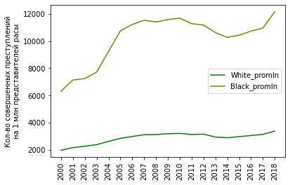
1. plt = df_arrests_2010_2018_agg.loc[:, ['white', 'black']].sort_index(ascending=False).plot.barh(color=['g', 'olive'], figsize=(10, 20))
   plt.set_ylabel('')
   plt.set_xlabel(' -  (2010-2018 .)')

2. :

plt = df_arrests_2010_2018_agg.loc[:, ['white_arrests_promln', 'black_arrests_promln']].sort_index(ascending=False).plot.barh(color=['g', 'olive'], figsize=(10, 20))
plt.set_ylabel('')
plt.set_xlabel(' -   1    (2010-2018 .)')

?

-, , - .

-, . "", , (. , , , .) -, ( , , , , , .

-, ( ) , .

.

:

df_arrests_2010_2018['white'].mean() / df_arrests_2010_2018['black'].mean()

- 1.56. .. 9 , .

:

df_arrests_2010_2018['white_arrests_promln'].mean() / df_arrests_2010_2018['black_arrests_promln'].mean()

- 0.183. .. 5.5 , .

, .

, , .

:

df_fenc_agg_states1 = df_fenc.merge(df_state_names, how='inner', left_on='State', right_on='state_abbr')
df_fenc_agg_states1.fillna(0, inplace=True)
df_fenc_agg_states1 = df_fenc_agg_states1.rename(columns={'state_name_x': 'state_name', 'Year': 'year'})
df_fenc_agg_states1 = df_fenc_agg_states1.loc[df_fenc_agg_states1['year'].between(2000, 2018), ['year', 'Race', 'state_name', 'UOF']]
df_fenc_agg_states1 = df_fenc_agg_states1.groupby(['year', 'state_name', 'Race'])['UOF'].count().unstack().reset_index()
df_fenc_agg_states1 = df_fenc_agg_states1.rename(columns={'Black': 'black_uof', 'White': 'white_uof'})
df_fenc_agg_states1 = df_fenc_agg_states1.fillna(0).astype({'black_uof': 'uint32', 'white_uof': 'uint32'})

:

df_arrests_fenc = df_arrests.merge(df_fenc_agg_states1, on=['state_name', 'year'])
df_arrests_fenc = df_arrests_fenc.rename(columns={'white': 'white_arrests', 'black': 'black_arrests'})

, , :

df_corr = df_arrests_fenc.loc[:, ['white_arrests', 'black_arrests', 'white_uof', 'black_uof']].corr(method='pearson').iloc[:2, 2:]
df_corr.style.background_gradient(cmap='PuBu')

: 0.87 0.77 ! , , ( 0.88 0.72 ).

, " ", :

df_arrests_fenc['white_uof_by_arr'] = df_arrests_fenc['white_uof'] / df_arrests_fenc['white_arrests']
df_arrests_fenc['black_uof_by_arr'] = df_arrests_fenc['black_uof'] / df_arrests_fenc['black_arrests']
df_arrests_fenc.replace([np.inf, -np.inf], np.nan, inplace=True)
df_arrests_fenc.fillna({'white_uof_by_arr': 0, 'black_uof_by_arr': 0}, inplace=True)

, ( 2018 ):

plt = df_arrests_fenc.loc[df_arrests_fenc['year'] == 2018, ['state_name', 'white_uof_by_arr', 'black_uof_by_arr']].sort_values(by='state_name', ascending=False).plot.barh(x='state_name', color=['g', 'olive'], figsize=(10, 20))
plt.set_ylabel('')
plt.set_xlabel(' -   -  ( 2018 .)')

, , : , , , .

:

plt = df_arrests_fenc.loc[:, ['white_uof_by_arr', 'black_uof_by_arr']].mean().plot.bar(color=['g', 'olive'])
plt.set_ylabel(' -   - ')
plt.set_xticklabels(['', ''], rotation=0)

2.5 . , - , 2.5 , . , : , 2 , - 4 .

, . .

1. . "" , , - . ( ) - , ( ) -.

2. ( ), .

3. : 3 5 , .

4. 2.5 , .

5. : , . , . : , .

, :)

PS. Im nächsten, separaten Artikel werde ich mich weiterhin mit der Kriminalität in den Vereinigten Staaten und ihrer Beziehung zur Rasse befassen. Lassen Sie uns zunächst mit den offiziellen Daten zu Verbrechen spielen, die durch Rassen- und andere Intoleranz motiviert sind, und dann werden wir die Konflikte zwischen der Polizei und der Bevölkerung von der anderen Seite untersuchen und die Fälle von Todesfällen durch die Polizei im Dienst analysieren. Wenn dieses Thema interessant ist, lass es mich bitte in den Kommentaren wissen!

Link zur englischen Version des Artikels  (auf Anfrage der Arbeiter).